Lesson 1b: Qwen3 Fundamentals
How a language model lives on disk and loads into memory — byte by byte.
Qwen3 Fundamentals
How a language model lives on disk and loads into memory — byte by byte.
This lesson ships in three video parts. Part A is live — run Qwen3 locally in pure C on your laptop or desktop. Parts B and C are on the way. The full written lesson below covers the file and memory layer in depth; the video mirrors it part by part. Click any transcript line to jump the video to that moment.
Chapter 1: What Even Is a Model File?
When someone says “I downloaded Qwen3-0.6B,” what did they actually get?
They got a file — typically 1–3 GB in size — that contains numbers. Millions and millions of numbers. These numbers are the weights (also called parameters) of the neural network. They were determined during training, and they encode everything the model “knows.”
Think of it like this:
- A recipe tells you the structure: “mix flour, eggs, and sugar, then bake at 350°F.”
- The ingredient amounts tell you the specifics: “2 cups flour, 3 eggs, 1.5 cups sugar.”
In a language model:
- The architecture is the recipe: “do attention, then feed-forward, repeat 28 times.”
- The weights are the ingredient amounts: the specific numbers that make this particular model produce coherent text.
The architecture is described by code (like our run.c). The weights are stored in a model file (the .gguf file). To do inference (generate text), you need both.
How Many Numbers Are We Talking About?
Qwen3-0.6B has approximately 600 million parameters. Each parameter is a 32-bit floating-point number (in our case), which takes 4 bytes. So:
600,000,000 parameters × 4 bytes each = 2,400,000,000 bytes ≈ 2.4 GBThat’s what takes up most of the model file. The rest is metadata (a tiny fraction by comparison).
What Does “Inference” Mean?
Inference is the process of using a trained model to generate predictions. For a language model, inference means: given some text (the prompt), generate the next token (word/subword), then the next, then the next, one at a time.
Every time the model generates one token, it performs hundreds of matrix multiplications using those 600 million numbers. That’s why inference, even for a “small” model, requires significant compute.
Chapter 2: The GGUF File Format — A Container for Brains
The Problem GGUF Solves
Imagine you’re given a file that’s just 2.4 billion raw bytes. You know they’re model weights, but:
- Where does the token embedding end and the attention weights begin?
- How many layers does this model have?
- What’s the vocabulary size?
- Is this Qwen3, LLaMA, or Mistral?
Without metadata, the file is just a soup of numbers. You’d need a separate config file, a separate tokenizer file, and exact knowledge of the weight layout to make any sense of it.
GGUF (GGML Universal Format) solves this by being a self-contained file format. One single .gguf file holds:
- Everything about the model’s architecture (number of layers, embedding size, etc.)
- The tokenizer (vocabulary, merge rules for BPE)
- Every single weight tensor with its name, shape, and data type
- The raw weight data itself
The Four Regions of a GGUF File
Every GGUF file is divided into four sequential regions, one after the other:
Byte 0                                                          Last byte
|                                                                       |
v                                                                       v
+----------+------------------+------------------+---------+------------+
|  HEADER  |  METADATA BLOCK  |  TENSOR INFO     | PADDING | TENSOR DATA|
| (24 bytes|  (variable size) |  (variable size) |         | (the big   |
|  fixed)  |                  |                  |         |  part)     |
+----------+------------------+------------------+---------+------------+
Let’s walk through each one.
Region 1: The Header (24 bytes, fixed)
The very first 24 bytes of every GGUF file are always structured the same way:
| Bytes | What It Is | Example Value |
|---|---|---|
| 0–3 | Magic number | GGUF (the ASCII characters G, G, U, F) |
| 4–7 | Version number | 3 (the current GGUF spec version) |
| 8–15 | Tensor count | 311 (how many weight tensors are in this file) |
| 16–23 | Metadata KV count | 34 (how many metadata key-value pairs follow) |
The magic number is a signature that lets any program quickly verify “yes, this is a GGUF file” before trying to parse it. If the first four bytes aren’t GGUF, something is wrong.
You can see these exact values in our header.txt file (which was generated by header.py parsing the binary GGUF):
MAGIC=GGUF
VERSION=3
TENSOR_COUNT=311
METADATA_COUNT=34
Region 2: The Metadata Block (variable size)
Immediately after the 24-byte header comes a series of key-value pairs. Each pair has:
- A key (a string, like
"qwen3.block_count") - A value type (integer, float, string, array, etc.)
- A value (the actual data)
For our Qwen3-0.6B model, the 34 metadata entries include things like:
GENERAL_ARCHITECTURE    = qwen3          (what kind of model this is)
GENERAL_NAME            = Qwen3 0.6B     (human-readable name)
QWEN3_BLOCK_COUNT       = 28             (number of transformer layers)
QWEN3_EMBEDDING_LENGTH  = 1024           (the "dimension" of the model)
QWEN3_FEED_FORWARD_LENGTH = 3072         (hidden dimension in FFN layers)
QWEN3_ATTENTION_HEAD_COUNT = 16          (number of attention heads)
QWEN3_ATTENTION_HEAD_COUNT_KV = 8        (number of key/value heads — GQA!)
QWEN3_ROPE_FREQ_BASE    = 1000000.0      (base frequency for positional encoding)
QWEN3_ATTENTION_KEY_LENGTH = 128         (dimension per attention head)
TOKENIZER_GGML_MODEL    = gpt2           (tokenizer type — BPE)
TOKENIZER_GGML_TOKENS   = [151936 strings] (the full vocabulary!)
TOKENIZER_GGML_MERGES   = [151387 strings] (BPE merge rules!)
This is incredibly powerful. A program reading this file can learn everything it needs to know about the model without any external files. It knows it’s a Qwen3 model with 28 layers, 1024-dimensional embeddings, 16 attention heads, and a vocabulary of 151,936 tokens — all from the file itself.
Region 3: The Tensor Info Block (variable size)
After all the metadata comes a directory listing of every tensor in the file. For each of the 311 tensors, the file stores:
| Field | What It Means | Example |
|---|---|---|
| Name | The tensor’s standardized name | "blk.0.attn_q.weight" |
| Number of dimensions | How many axes the tensor has | 2 (a matrix) |
| Dimensions | The size along each axis | [1024, 2048] |
| Type | The data type / quantization format | 0 (= F32, 32-bit float) |
| Offset | Where this tensor’s data starts within the data blob | 1257251328 |
This is like a table of contents for the weights. It tells you: “the Q projection for layer 0 is a 1024×2048 matrix of 32-bit floats, and its data starts at byte offset 1,257,251,328 within the tensor data region.”
Region 4: Padding + Tensor Data (the bulk of the file)
After the tensor info block, there’s some padding (zero bytes) to align the start of the data to a 32-byte boundary. Then comes the actual weight data — just raw numbers, one after another.
Why 32-byte alignment? Modern CPUs have special instructions (called SIMD — Single Instruction, Multiple Data) that can process 8 floats at once, but only if the data starts at a memory address that’s a multiple of 32. Alignment ensures that when the file is memory-mapped (we’ll explain this in Chapter 4), the weights are already perfectly aligned for fast math.
Chapter 3: Our Qwen3 GGUF File — A Concrete Example
Let’s look at the actual tensor layout in our Qwen3-0.6B GGUF file. The header.txt file (generated by header.py) shows us every tensor.
The Global Tensors (Not Part of Any Layer)
The first three tensors are the “global” ones — they don’t belong to any specific transformer layer:
TENSOR_0:  OUTPUT_WEIGHT         shape=[1024, 151936]  offset=0
TENSOR_1:  OUTPUT_NORM_WEIGHT    shape=[1024]           offset=622,329,856
TENSOR_2:  TOKEN_EMBD_WEIGHT     shape=[1024, 151936]  offset=622,333,952
OUTPUT_WEIGHT (also called wcls in the code, or the “LM head”): This is the very last matrix multiplication in the model. It takes the model’s internal representation (a 1024-dimensional vector) and projects it to a probability distribution over all 151,936 tokens in the vocabulary. Size: 1024 × 151,936 = 155,582,464 floats = 622,329,856 bytes.
OUTPUT_NORM_WEIGHT: A small 1024-element vector used for RMSNorm right before the output projection. Just 4,096 bytes.
TOKEN_EMBD_WEIGHT (the token embedding table): This is the very first thing used in the model. When a token comes in (say, token ID 5032), we look up row 5032 in this table to get a 1024-dimensional vector. Same size as OUTPUT_WEIGHT: 1024 × 151,936.
The Per-Layer Tensors (Repeated 28 Times)
Starting from TENSOR_3, we see the same pattern repeat for each of the 28 transformer layers. Here’s layer 0 (block 0):
TENSOR_3:   BLK_0_ATTN_K_WEIGHT          [1024, 1024]   — Key projection
TENSOR_4:   BLK_0_ATTN_K_NORM_WEIGHT     [128]           — Key RMSNorm
TENSOR_5:   BLK_0_ATTN_NORM_WEIGHT       [1024]          — Pre-attention RMSNorm
TENSOR_6:   BLK_0_ATTN_OUTPUT_WEIGHT     [2048, 1024]    — Attention output projection
TENSOR_7:   BLK_0_ATTN_Q_WEIGHT          [1024, 2048]    — Query projection
TENSOR_8:   BLK_0_ATTN_Q_NORM_WEIGHT     [128]           — Query RMSNorm
TENSOR_9:   BLK_0_ATTN_V_WEIGHT          [1024, 1024]    — Value projection
TENSOR_10:  BLK_0_FFN_DOWN_WEIGHT        [3072, 1024]    — FFN down projection
TENSOR_11:  BLK_0_FFN_GATE_WEIGHT        [1024, 3072]    — FFN gate projection
TENSOR_12:  BLK_0_FFN_NORM_WEIGHT        [1024]          — Pre-FFN RMSNorm
TENSOR_13:  BLK_0_FFN_UP_WEIGHT          [1024, 3072]    — FFN up projection
That’s 11 tensors per layer. With 28 layers, that’s 308 per-layer tensors, plus 3 global tensors = 311 total. Exactly matching our TENSOR_COUNT=311.
Important observation: Within each block, the tensors are in alphabetical order by their GGUF name: attn_k, attn_k_norm, attn_norm, attn_output, attn_q, attn_q_norm, attn_v, ffn_down, ffn_gate, ffn_norm, ffn_up. This is not the order llama.cpp normally uses — this is a deliberate choice made by our custom conversion script, and it’s essential for our loading code to work. We’ll explain why in Chapter 6.
Understanding the Shapes
Let’s decode what each tensor’s shape means for Qwen3-0.6B:
- dim = 1024 (the model’s internal working dimension)
- n_heads = 16 (number of attention heads)
- n_kv_heads = 8 (number of key/value heads — this is Grouped Query Attention)
- head_dim = 128 (each head works with 128-dimensional vectors; 16 heads × 128 = 2048)
- hidden_dim = 3072 (the expanded dimension inside the FFN)
So:
ATTN_Q_WEIGHT [1024, 2048]: Projects a 1024-dim input to a 2048-dim query vector (16 heads × 128 per head)ATTN_K_WEIGHT [1024, 1024]: Projects 1024-dim input to a 1024-dim key vector (8 KV heads × 128 per head)ATTN_V_WEIGHT [1024, 1024]: Same as K (8 KV heads × 128 per head)ATTN_OUTPUT_WEIGHT [2048, 1024]: Projects the 2048-dim attention output back to 1024-dimFFN_UP_WEIGHT [1024, 3072]: Expands 1024 → 3072FFN_DOWN_WEIGHT [3072, 1024]: Compresses 3072 → 1024
Chapter 4: Memory Mapping — Opening the File Without Reading It
The Naive Approach (and Why It’s Bad)
The obvious way to load a 2.4 GB model file would be:
// DON'T do this for large files
FILE *f = fopen("model.gguf", "rb");
char *buffer = malloc(2400000000);  // allocate 2.4 GB of RAM
fread(buffer, 1, 2400000000, f);    // read entire file into RAM
fclose(f);
This works, but it has problems:
- It uses 2.4 GB of RAM just for the weights. Your program also needs RAM for activations, KV cache, etc.
- It’s slow to start — you have to read the entire file from disk before you can do anything.
- It makes a copy — the data exists on disk AND in RAM, doubling the effective memory usage from the OS’s perspective.
The Memory Mapping Approach
Memory mapping (mmap) is an operating system feature that creates a virtual window into a file. Instead of reading the file into RAM, you tell the OS: “make this file appear as if it were already in my memory.”
// What our run.c actually does
int fd = open("model.gguf", O_RDONLY);      // open the file
void *data = mmap(NULL, file_size,           // create a memory mapping
                  PROT_READ, MAP_PRIVATE,
                  fd, 0);
After this call, data is a pointer. You can read data[0], data[1000], data[2000000000] — any byte in the file — and the OS handles the rest. Here’s what’s actually happening behind the scenes:
- No data is loaded yet. The
mmapcall returns almost instantly. It just sets up address space. - When you access a byte, the OS loads just that 4 KB page from disk into RAM (this is called a “page fault,” but it’s normal and fast).
- Pages you don’t access are never loaded. If there are tensors you never use, their data stays on disk.
- The OS manages the memory. If RAM gets tight, the OS can evict mapped pages and reload them later from disk, since the file is the backing store.
This is why mmap is the standard way to load model weights in inference engines. For our 2.4 GB model:
- Startup is nearly instant (just a system call, no data movement)
- Memory efficient (only pages actually accessed are in RAM)
- Zero-copy (we read directly from the OS page cache — no duplicate in application memory)
Here’s the actual code from run.c:
void read_checkpoint(char *checkpoint, Config *config, TransformerWeights* weights,
                     int* fd, float** data, ssize_t* file_size) {
    FILE *file = fopen(checkpoint, "rb");
    fseek(file, 0, SEEK_END);
    *file_size = (ssize_t)ftell(file);    // get total file size
    fclose(file);

    *fd = open(checkpoint, O_RDONLY);
    *data = mmap(NULL, *file_size, PROT_READ, MAP_PRIVATE, *fd, 0);

    void* weights_ptr = ((char*)*data) + 5951648;  // skip header to reach tensor data
    memory_map_weights(weights, config, weights_ptr);
}
Let’s break that down line by line:
- Open the file just to get its size (
fseekto end,ftellto read position), then close it - Open the file again with
open()(the low-level system call, needed formmap) - Call
mmap()to create the memory mapping over the entire file - Calculate
weights_ptrby skipping past the header to reach the raw weight data - Call
memory_map_weights()to set up pointers to each weight tensor
Chapter 5: The Header Skip — Jumping to the Weights
The Problem
After memory-mapping the GGUF file, the pointer data points to the very beginning of the file — the magic number GGUF. But we don’t want to do math with the string “GGUF”. We want the actual weight numbers, which are in Region 4 (the tensor data blob), thousands of bytes into the file.
We need to figure out: how many bytes do we skip to reach the tensor data?
Where the Number 5,951,648 Comes From
In our code, the skip is hardcoded:
void* weights_ptr = ((char*)*data) + 5951648;This number was calculated from the GGUF file itself. Here’s the logic:
The tensor info block in our header.txt tells us that the last tensor (TENSOR_310, which is BLK_27_FFN_UP_WEIGHT) has:
TENSOR_310_DIMENSIONS=1024,3072
TENSOR_310_TYPE=0          (F32 = 4 bytes per number)
TENSOR_310_OFFSET=2993946624
The offset tells us this tensor’s data starts at byte 2,993,946,624 relative to the start of the tensor data blob. Its size is 1024 × 3072 × 4 bytes = 12,582,912 bytes. So the total tensor data size is:
tensor_data_size = last_offset + last_tensor_size
                 = 2,993,946,624 + 12,582,912
                 = 3,006,529,536 bytes
And the header size (everything before the tensor data) is:
header_size = total_file_size - tensor_data_size
            = 3,012,481,184 - 3,006,529,536
            = 5,951,648 bytes
That’s where the magic number 5951648 comes from. It represents:
- 24 bytes of GGUF header
- Several thousand bytes of metadata (34 key-value pairs, including the huge tokenizer vocabulary and merge tables)
- Several thousand bytes of tensor info (311 tensor descriptions)
- A few bytes of padding for alignment
Why This Is “Fragile” (and That’s OK for Learning)
This hardcoded number is correct only for this exact file. If you:
- Used a model with a different vocabulary size (the tokenizer arrays in the metadata would be different sizes)
- Used a model with more or fewer layers (different number of tensor info entries)
- Changed any metadata field
…the header size would change, and 5,951,648 would be wrong. The code would point to the wrong place and the model would produce garbage (or crash).
In a production system like llama.cpp, this offset is calculated dynamically by actually parsing the header. But for learning, the hardcoded value lets us focus on what matters: understanding the tensor data itself.
The comment in the code even acknowledges this with a TODO:
void* weights_ptr = ((char*)*data) + 5951648; // skip header bytes. header_size = 5951648 TODOChapter 6: memory_map_weights() — The Pointer Walk
This is the heart of the weight-loading logic, and it’s worth understanding in extreme detail.
The Setup
After skipping the header, weights_ptr points to the very first byte of the tensor data blob. We know from our header.txt that the tensors are laid out in this order:
[OUTPUT_WEIGHT][OUTPUT_NORM_WEIGHT][TOKEN_EMBD_WEIGHT][BLK_0_ATTN_K][BLK_0_ATTN_K_NORM]...All the numbers are 32-bit floats (4 bytes each), packed tightly together (with alignment padding between some tensors).
The Code, Fully Annotated
void memory_map_weights(TransformerWeights* w, Config* p, void* pt) {
    unsigned long long n_layers = p->n_layers;  // = 28
    float *ptr = (float*) pt;   // Cast the raw byte pointer to a float pointer
                                // Now ptr[0] is the first float, ptr[1] is the second, etc.

    // --- TENSOR 0: output.weight (wcls) ---
    // Shape: [1024, 151936] = 155,582,464 floats
    w->wcls = ptr;
    ptr += p->vocab_size * p->dim;      // advance by 151936 * 1024 = 155,582,464 floats

    // --- TENSOR 1: output_norm.weight (rms_final_weight) ---
    // Shape: [1024] = 1,024 floats
    w->rms_final_weight = ptr;
    ptr += p->dim;                       // advance by 1024 floats

    // --- TENSOR 2: token_embd.weight ---
    // Shape: [1024, 151936] = 155,582,464 floats
    w->token_embedding_table = ptr;
    ptr += p->vocab_size * p->dim;      // advance by 155,582,464 floats

    // --- TENSOR 3: blk.0.attn_k.weight ---
    // Shape: [1024, 1024] (dim × n_kv_heads * head_dim = 1024 × 8*128)
    w->wk = ptr;
    ptr += p->dim * (p->n_kv_heads * p->head_dim);

    // --- TENSOR 4: blk.0.attn_k_norm.weight ---
    // Shape: [128] (one per head_dim)
    w->wk_norm = ptr;
    ptr += p->head_dim;

    // --- TENSOR 5: blk.0.attn_norm.weight (pre-attention RMSNorm) ---
    // Shape: [1024]
    w->rms_att_weight = ptr;
    ptr += p->dim;

    // --- TENSOR 6: blk.0.attn_output.weight ---
    // Shape: [2048, 1024] (n_heads * head_dim × dim)
    w->wo = ptr;
    ptr += (p->n_heads * p->head_dim) * p->dim;

    // --- TENSOR 7: blk.0.attn_q.weight ---
    // Shape: [1024, 2048] (dim × n_heads * head_dim)
    w->wq = ptr;
    ptr += p->dim * (p->n_heads * p->head_dim);

    // --- TENSOR 8: blk.0.attn_q_norm.weight ---
    // Shape: [128]
    w->wq_norm = ptr;
    ptr += p->head_dim;

    // --- TENSOR 9: blk.0.attn_v.weight ---
    // Shape: [1024, 1024] (dim × n_kv_heads * head_dim)
    w->wv = ptr;
    ptr += p->dim * (p->n_kv_heads * p->head_dim);

    // --- TENSOR 10: blk.0.ffn_down.weight (w2) ---
    // Shape: [3072, 1024] (hidden_dim × dim)
    w->w2 = ptr;
    ptr += p->hidden_dim * p->dim;

    // --- TENSOR 11: blk.0.ffn_gate.weight (w3) ---
    // Shape: [1024, 3072] (dim × hidden_dim)
    w->w3 = ptr;
    ptr += p->dim * p->hidden_dim;

    // --- TENSOR 12: blk.0.ffn_norm.weight (pre-FFN RMSNorm) ---
    // Shape: [1024]
    w->rms_ffn_weight = ptr;
    ptr += p->dim;

    // --- TENSOR 13: blk.0.ffn_up.weight (w1) ---
    // Shape: [1024, 3072] (dim × hidden_dim)
    w->w1 = ptr;
    ptr += p->dim * p->hidden_dim;

    // ptr now points to TENSOR 14: blk.1.attn_k.weight
    // But the function ends here! It only recorded the pointer to layer 0.
    // The forward pass accesses other layers using an offset. See Chapter 7.
}
What Just Happened?
We walked a pointer through memory, assigning each weight struct member to point to the correct location in the memory-mapped file. No data was copied. Each w->something is just a pointer to a position within the mmap’d file.
Here’s a visual of what memory looks like after this function:
Memory-mapped file (starting from tensor data):

Byte 0                                                    Byte ~3 billion
|                                                                      |
v                                                                      v
[output.weight ......][norm][token_embd ......][blk0.attn_k][blk0.k_norm]...
^                      ^     ^                  ^            ^
|                      |     |                  |            |
w->wcls          w->rms_final w->token_embd    w->wk        w->wk_norm
Each pointer is essentially a bookmark into this giant contiguous block of memory. When the forward pass needs to do a matrix multiplication with the Q projection weights, it just uses w->wq — which is already pointing at the right spot in the file.
The Critical Requirement: Order Must Match
This entire scheme depends on the tensors being physically laid out in the file in exactly the order that memory_map_weights() expects. If output_norm.weight came before output.weight in the file, the pointer walk would assign wrong sizes and every subsequent pointer would be in the wrong place. The model would produce garbage.
This is why we use the custom convert_hf_to_gguf_ordered.py script instead of the standard llama.cpp converter. Our script sorts the tensors into the exact order our code expects.
Chapter 7: How the Forward Pass Uses These Pointers
The Layer Offset Trick
memory_map_weights() only stored pointers to layer 0’s weights. But Qwen3-0.6B has 28 layers. How does the forward pass access layer 5, or layer 27?
The answer is a constant called layer_offset:
int layer_offset = 62923776 / 4; // = 15,730,944 floatsThis is the stride between consecutive layers’ tensors of the same type. Because our GGUF file arranges tensors as [all of block 0, all of block 1, all of block 2, …], and every block has the exact same sizes, the distance from blk.0.attn_k.weight to blk.1.attn_k.weight is always the same.
That distance is 62,923,776 bytes (= the total size of all 11 tensors in one block). Divided by 4 (bytes per float) = 15,730,944 floats.
So to access layer l’s Q projection weights, the code does:
w->wq + l * layer_offsetThis is pointer arithmetic: “start at layer 0’s wq, then jump forward by l blocks.”
Walking Through One Forward Pass Layer
Here’s the forward pass for one layer, annotated:
for (int l = 0; l < p->n_layers; l++) {     // for each of the 28 layers

    // Step 1: RMSNorm the input (normalize before attention)
    rmsnorm(s->xb, s->x, w->rms_att_weight + l * layer_offset, p->dim);

    // Step 2: Compute Q, K, V projections
    matmul(s->q, s->xb, w->wq + l * layer_offset, p->dim, att_head_dim);
    matmul(s->k, s->xb, w->wk + l * layer_offset, p->dim, kv_dim);
    matmul(s->v, s->xb, w->wv + l * layer_offset, p->dim, kv_dim);

    // Step 3: Apply QK norms (Qwen3-specific!)
    rmsnorm(q, q, w->wq_norm + l * layer_offset, p->head_dim);
    rmsnorm(k, k, w->wk_norm + l * layer_offset, p->head_dim);

    // Step 4: Apply RoPE (Rotary Position Embedding)
    // ... (rotates q and k vectors based on position)

    // Step 5: Attention (dot product of Q and K, softmax, weighted sum of V)
    // ... (the classic attention mechanism)

    // Step 6: Output projection
    matmul(s->xb2, s->xb3, w->wo + l * layer_offset, att_head_dim, p->dim);

    // Step 7: Residual connection (add attention output back to input)
    for (int i = 0; i < p->dim; i++)
        s->x[i] += s->xb2[i];

    // Step 8: FFN RMSNorm
    rmsnorm(s->xb, s->x, w->rms_ffn_weight + l * layer_offset, p->dim);

    // Step 9: FFN (SwiGLU activation)
    matmul(s->hb,  s->xb, w->w1 + l * layer_offset, p->dim, p->hidden_dim);  // up
    matmul(s->hb2, s->xb, w->w3 + l * layer_offset, p->dim, p->hidden_dim);  // gate
    // SwiGLU: gate * silu(up), then project down
    matmul(s->xb, s->hb2, w->w2 + l * layer_offset, p->hidden_dim, p->dim);  // down

    // Step 10: Residual connection (add FFN output back)
    for (int i = 0; i < p->dim; i++)
        s->x[i] += s->xb[i];
}
After all 28 layers, one final step:
// Final RMSNorm
rmsnorm(s->x, s->x, w->rms_final_weight, p->dim);

// Project to vocabulary-sized logits
matmul(s->logits, s->x, w->wcls, p->dim, p->vocab_size);
The logits array now has 151,936 values — one score for every possible next token. The highest-scoring token (or a sampled one) becomes the model’s output.
Chapter 8: Inside the Transformer Layer — Attention and the MLP
Chapter 7 showed you the forward pass as code — ten steps per layer. But why does each layer have this structure? Each of the 28 layers in Qwen3-0.6B has two main blocks:
Transformer Layer
 ├── Attention block       ← tokens talk to each other
 │    ├── q_proj (wq)
 │    ├── k_proj (wk)
 │    ├── v_proj (wv)
 │    └── o_proj (wo)
 │
 └── MLP / FFN block       ← each token refines its own representation
      ├── gate_proj (w3)
      ├── up_proj (w1)
      └── down_proj (w2)
Attention mixes information across tokens (“which other tokens should I look at?”). The MLP transforms each token’s representation independently (“after seeing the context, how should I update this token’s meaning?”). Both are required — one without the other is insufficient.
Multi-Head Attention — Why 16 Smaller Views Beat One Big One
Single-head attention (the starting point)
In the simplest version, each token gets one query, one key, and one value — all of size dim (1024). The attention score is a single dot product between Q and K, and the output is a single weighted sum of V. This gives each token one way of looking at the sequence.
The problem with one head
A token often needs to attend to different things simultaneously. Consider:
"The animal didn't cross the road because it was tired."For the token “it”, the model needs to:
- Connect “it” to “animal” (coreference)
- Track negation from “didn’t” (semantics)
- Understand “tired” as a state (predicate)
- Recognize phrase boundaries (syntax)
One attention pattern can’t do all of this at once. It produces one set of attention weights — one “view” of the sequence.
Multi-head: many smaller views in parallel
Instead of one big attention with 1024-dimensional Q, K, V, the model splits them into 16 heads of 128 dimensions each:
hidden_size = 1024
n_heads     = 16
head_dim    = 1024 / 16 = 64... wait — Qwen3 uses head_dim = 128
Qwen3’s head_dim is 128, not 1024/16 = 64. So the full Q projection output is actually n_heads × head_dim = 16 × 128 = 2048, which is larger than the hidden size. This is why wq has shape [2048, 1024] — it projects 1024-dim input into 2048-dim Q space.
Step by step in run.c
Step 1: Create Q, K, V. The projections produce the full output:
matmul(s->q, s->xb, w->wq + l * layer_offset, p->dim, att_head_dim);
// s->q shape: [2048] = 16 heads × 128 dim per head

matmul(s->k, s->xb, w->wk + l * layer_offset, p->dim, kv_dim);
// s->k shape: [1024] = 8 KV heads × 128 dim per head (GQA!)
Step 2: Split into heads. The code doesn’t explicitly reshape — it uses pointer arithmetic. Each head’s Q is a slice of 128 floats:
for (int h = 0; h < p->n_heads; h++) {
    float* q = s->q + h * p->head_dim;  // head 0: q[0..127], head 1: q[128..255], ...
This is the “reshape” that frameworks like PyTorch do with view() and transpose() — but in C, it’s just a pointer offset.
Step 3: Each head does independent attention. Every head computes its own attention scores (dot products of Q with all past K vectors), applies softmax, and produces a weighted sum of V:
    float* att = s->att + h * p->seq_len;  // this head's score buffer

    for (int t = 0; t <= pos; t++) {
        float* k = s->key_cache + loff + t * kv_dim + (h / kv_mul) * p->head_dim;
        float score = 0;
        for (int i = 0; i < p->head_dim; i++)
            score += q[i] * k[i];
        att[t] = score / sqrtf(p->head_dim);
    }
    softmax(att, pos + 1);

    // weighted sum of values
    float* xb3 = s->xb3 + h * p->head_dim;
    memset(xb3, 0, p->head_dim * sizeof(float));
    for (int t = 0; t <= pos; t++) {
        float* v = s->value_cache + loff + t * kv_dim + (h / kv_mul) * p->head_dim;
        float a = att[t];
        for (int i = 0; i < p->head_dim; i++)
            xb3[i] += a * v[i];
    }
}
Each head produces 128 floats. 16 heads × 128 = 2048 floats total, sitting contiguously in s->xb3.
Step 4: Output projection. The o_proj (w->wo) mixes information across heads and projects back to 1024 dimensions:
matmul(s->xb2, s->xb3, w->wo + l * layer_offset, att_head_dim, p->dim);
// [2048] → [1024]
Without o_proj, the head outputs would remain separated — head 0’s 128 floats wouldn’t interact with head 7’s 128 floats. The output projection lets the model combine what different heads learned.
The full picture
Input x [1024]
     │
     ├─→ wq ─→ Q [2048] ─→ split into 16 heads of [128]
     ├─→ wk ─→ K [1024] ─→ split into  8 heads of [128] (GQA)
     └─→ wv ─→ V [1024] ─→ split into  8 heads of [128] (GQA)
                                │
                    ┌───────────┼───────────┐
                 Head 0      Head 1  ...  Head 15
                attention   attention    attention
                 [128]       [128]        [128]
                    └───────────┼───────────┘
                                │
                          concatenate [2048]
                                │
                         wo (o_proj) [2048 → 1024]
                                │
                    + residual connection
                                │
                          Output x [1024]
Each head can learn a different relationship. Head 3 might track coreference while head 11 tracks syntactic structure. The model doesn’t assign these roles explicitly — the heads discover useful patterns during training.
The MLP Block — Up, Gate, and Down Projections
After attention, each token has gathered context from the sequence. Now the MLP transforms each token’s representation independently — no cross-token communication.
Why not just 1024 → 1024?
A direct projection from 1024 to 1024 is limited. The MLP expands to a larger internal space, works in that space, and compresses back:
1024 → 3072 → 1024This is like solving a problem by expanding your working space, doing the reasoning, then compressing the final result. The larger intermediate dimension gives the network more expressive capacity to represent complex patterns.
The three projections in Qwen3
Qwen3 uses a gated MLP (SwiGLU style) with three projections:
| Projection | run.c name |
Shape | Role |
|---|---|---|---|
up_proj |
w->w1 |
[1024, 3072] | Expand to candidate features |
gate_proj |
w->w3 |
[1024, 3072] | Control which features pass |
down_proj |
w->w2 |
[3072, 1024] | Compress back to hidden size |
The computation:
x ──→ gate_proj ──→ SiLU activation ──┐
                                       × ──→ down_proj ──→ output
x ──→ up_proj ────────────────────────┘
Or as a formula: output = down_proj( SiLU(gate_proj(x)) × up_proj(x) )
The code in run.c
// up_proj: x [1024] → hb [3072]
matmul(s->hb, s->xb, w->w1 + l * layer_offset, p->dim, p->hidden_dim);

// gate_proj: x [1024] → hb2 [3072]
matmul(s->hb2, s->xb, w->w3 + l * layer_offset, p->dim, p->hidden_dim);

// SwiGLU: silu(gate) * up
for (int i = 0; i < p->hidden_dim; i++) {
    float val = s->hb2[i];
    val *= (1.0f / (1.0f + expf(-val)));  // silu(x) = x * sigmoid(x)
    val *= s->hb[i];                       // elementwise multiply with up_proj
    s->hb2[i] = val;
}

// down_proj: [3072] → [1024]
matmul(s->xb, s->hb2, w->w2 + l * layer_offset, p->hidden_dim, p->dim);
The gate_proj acts as a learned filter. It decides which of the 3072 intermediate features matter for this token. up_proj creates the candidate features. The elementwise multiply combines them — features where the gate is near zero get suppressed, features where the gate is large pass through.
Intuition: the “bank” analogy
Suppose a token’s 1024-dim vector encodes the compressed meaning of "bank". Depending on context, it could mean a river bank, a money bank, a banking API, or a bank angle in aviation. The MLP expands this into 3072 dimensions — room to create intermediate features like “is this financial?”, “is this geographical?”, “is this code?” (not with human labels, but conceptually). The gate selects which features are relevant given the context that attention already gathered. Then down_proj compresses the refined representation back to 1024 for the next layer.
Why Both Blocks Are Needed
| Block | What it does | Operates on |
|---|---|---|
| Attention | Mixes information across tokens | All tokens in the sequence |
| MLP | Transforms features within each token | Each token independently |
Attention answers: “Which other tokens should I look at?”
The MLP answers: “After seeing the context, how should I update this token’s meaning?”
A model with only attention could gather context but couldn’t transform it. A model with only MLPs could transform tokens but each token would be isolated — unable to see anything else in the sequence. The alternating attention-MLP structure, repeated 28 times, builds increasingly sophisticated representations.
The Complete Layer Flow
Putting it all together — one of the 28 identical layers:
Input x [1024]
     │
     ├─→ RMSNorm
     │     │
     │     ├─→ Q, K, V projections
     │     ├─→ QK norms + RoPE (position encoding)
     │     ├─→ Multi-head attention (16 heads)
     │     └─→ o_proj [2048 → 1024]
     │              │
     ├── + ─────────┘  (residual connection)
     │
     ├─→ RMSNorm
     │     │
     │     ├─→ up_proj  [1024 → 3072]
     │     ├─→ gate_proj [1024 → 3072]
     │     ├─→ SwiGLU activation
     │     └─→ down_proj [3072 → 1024]
     │              │
     ├── + ─────────┘  (residual connection)
     │
Output x [1024]
The residual connections (s->x[i] += ...) are critical — they let the input pass through unchanged and only add what attention and the MLP learned. This makes deep networks trainable; without residuals, 28 layers of transformations would be nearly impossible to optimize.
Chapter 9: How llama.cpp Does It Differently
Now that you understand the “simple” approach in run.c, let’s see how the production-grade llama.cpp handles the same problem.
Name-Based Lookup Instead of Pointer Walking
llama.cpp does not assume any particular order of tensors in the file. Instead, it:
- Parses the GGUF header and metadata (dynamically, not from a separate text file)
- Reads the entire tensor info block, building a dictionary mapping tensor names to their offsets
- When it needs a tensor (like
blk.5.attn_q.weight), it looks up the name in the dictionary, gets the offset, and computes the pointer
This means the tensors could be in any order in the file and llama.cpp would still work. It’s like the difference between:
- run.c: “The milk is the third item on the second shelf” (positional — breaks if you rearrange the fridge)
- llama.cpp: “The milk is labeled ‘MILK’” (named — works regardless of where it’s placed)
Dynamic Header Parsing
llama.cpp reads the GGUF metadata directly from the binary file at startup. It doesn’t need a pre-generated header.txt. The parsing code:
- Reads the magic number and validates it
- Reads the version number
- Reads tensor count and metadata KV count
- Loops through each KV pair, reading keys and values based on their type codes
- Loops through each tensor info entry, recording name, shape, type, and offset
- Calculates the tensor data start position (after padding)
This means llama.cpp can load any GGUF file — Qwen3, LLaMA, Mistral, Phi, Gemma — without modification. The architecture-specific code only needs to know which tensor names to look for.
Quantization Support
This is one of the biggest practical differences. Our run.c only handles TYPE=0 (F32 — full 32-bit floats). llama.cpp supports many quantization formats:
| Type | Bits per Weight | Size of 0.6B Model | Quality Loss |
|---|---|---|---|
| F32 | 32 | ~2.4 GB | None (reference) |
| F16 | 16 | ~1.2 GB | Negligible |
| Q8_0 | 8 | ~0.6 GB | Very small |
| Q4_K_M | ~4.5 | ~0.35 GB | Small |
| Q4_0 | 4 | ~0.3 GB | Moderate |
| Q2_K | ~2.6 | ~0.2 GB | Noticeable |
Quantization dramatically reduces file size and memory usage, making it possible to run larger models on consumer hardware. A 7B model at Q4_K_M fits in about 4 GB of RAM. At F32, it would need 28 GB.
In GGUF, each tensor declares its own quantization type. Some tensors (like embeddings and norms) might be kept at higher precision (F32 or F16) while the bulk of attention and FFN weights are quantized to Q4 or Q8. llama.cpp’s inference code knows how to dequantize each format on the fly.
The Standard Tensor Naming Convention
llama.cpp standardizes tensor names across all model architectures. The convention is:
token_embd.weight              — Token embedding
output_norm.weight             — Final RMSNorm before output
output.weight                  — LM head (vocabulary projection)

blk.{i}.attn_norm.weight       — Pre-attention RMSNorm for layer i
blk.{i}.attn_q.weight          — Query projection for layer i
blk.{i}.attn_k.weight          — Key projection for layer i
blk.{i}.attn_v.weight          — Value projection for layer i
blk.{i}.attn_output.weight     — Attention output projection for layer i
blk.{i}.ffn_norm.weight        — Pre-FFN RMSNorm for layer i
blk.{i}.ffn_gate.weight        — FFN gate (for SwiGLU)
blk.{i}.ffn_up.weight          — FFN up projection
blk.{i}.ffn_down.weight        — FFN down projection
These names are different from the HuggingFace names (e.g., model.layers.0.self_attn.q_proj.weight). A mapping table (tensor_mapping.py) translates between the two during conversion.
Chapter 10: The Custom Conversion Script — Making the Two Worlds Meet
The Bridge Between HuggingFace and run.c
Our codebase includes convert_hf_to_gguf_ordered.py — a modified version of llama.cpp’s standard conversion script. This script takes a HuggingFace model (SafeTensors format) and produces a GGUF file that our run.c can load.
The standard llama.cpp script writes tensors in whatever order they come from the source files. Our modified version adds a sorting step.
The Sorting Logic
Here’s the key addition (in the prepare_tensors() method):
def sort_key(tensor_info):
    new_name, data_torch, name, bid, old_dtype = tensor_info
    if bid is None:
        return (-1, new_name)   # Global tensors first (output, norm, embedding)
    else:
        return (bid, new_name)  # Then block 0 (alphabetical), block 1, ...

all_tensors.sort(key=sort_key)
This sort produces exactly the tensor order that memory_map_weights() expects:
- Global tensors first (bid = None, sorted to -1):
output.weight,output_norm.weight,token_embd.weight(alphabetical by name) - Block 0 (bid = 0): all 11 tensors, alphabetically by GGUF name
- Block 1 (bid = 1): all 11 tensors, alphabetically
- … and so on through block 27
Why Alphabetical?
The alphabetical ordering within each block is what gives us the specific sequence: attn_k, attn_k_norm, attn_norm, attn_output, attn_q, attn_q_norm, attn_v, ffn_down, ffn_gate, ffn_norm, ffn_up. This happens to match the order in memory_map_weights() because that function was written to match this alphabetical layout.
The Full Pipeline
HuggingFace Model                    Our Custom GGUF              run.c
(SafeTensors + config.json)     (ordered, FP32, sorted)      (pointer walk)

model.safetensors  ──────>  convert_hf_to_gguf_ordered.py  ──>  Qwen3-0.6B-F32.gguf
config.json        ──────>       (sorts tensors!)
tokenizer files    ──────>

                                                             header.py ──> header.txt
                                                                              |
                                                             extract_v_m.py ──> vocab.txt
                                                                              |  merges.txt
                                                                              v
                                                             run.c reads header.txt for config,
                                                             mmaps the GGUF, walks pointers,
                                                             runs inference
Chapter 11: Putting It All Together — The Full Pipeline
Let’s trace the entire journey from “you have a model” to “it generates a token.”
Step 1: Convert the Model
python convert_hf_to_gguf_ordered.py /path/to/Qwen3-0.6B --outtype f32 --outfile Qwen3-0.6B-F32.ggufThis reads the HuggingFace model, maps tensor names to GGUF standard names, sorts them by block then alphabetically, and writes the GGUF file with all weights in F32.
Step 2: Extract the Header
python header.py Qwen3-0.6B-F32.ggufThis parses the GGUF binary header and writes header.txt — a human-readable version that run.c can parse for the model’s configuration (dimensions, layer count, etc.).
Step 3: Extract Vocabulary and Merges
python extract_v_m.py Qwen3-0.6B-F32.ggufThis extracts the BPE tokenizer data (vocab.txt and merges.txt) that run.c needs to convert text to token IDs and back.
Step 4: Compile and Run
gcc -O3 -o run run.c -lm
./run Qwen3-0.6B-F32.gguf
At startup, run.c:
- Calls
load_config()— readsheader.txtto fill theConfigstruct (dim=1024, n_layers=28, etc.) - Calls
build_transformer()which:- Opens the GGUF file and gets its size
- Memory-maps the entire file with
mmap() - Skips 5,951,648 bytes to reach the tensor data
- Walks the pointer through
memory_map_weights(), setting up all weight pointers - Allocates runtime buffers (activations, KV cache) with
malloc_run_state()
- Loads the tokenizer (vocabulary and merge rules from text files)
- Enters the generation loop:
- Encode the prompt text into token IDs
- For each position: call
forward()to get logits, sample a token, decode it to text - Print each generated token
The Beauty of This Design
Even though it’s simplified, this design captures the essential structure of every LLM inference engine:
- Load weights from a file (GGUF, SafeTensors, or raw binary)
- Point weight matrices at the data (via mmap, GPU upload, or copy)
- Run the transformer forward pass (embedding → [attention + FFN] × N layers → logits)
- Sample the next token (from the logit distribution)
- Repeat
The difference between this and llama.cpp or vLLM or TensorRT-LLM is one of flexibility and optimization (quantization, batching, GPU kernels, speculative decoding), not fundamental structure.
Chapter 12: SafeTensors — The Other File Format
In the previous chapters, we studied GGUF in detail. But when you download a model from HuggingFace, you don’t get a GGUF file. You get SafeTensors files. So what are those, and why do we need to convert them?
Why SafeTensors Was Created: A Security Story
Before SafeTensors existed, PyTorch models were stored as pickle files (.bin or .pt). Pickle is a Python serialization format, and here’s its dangerous secret: pickle can execute arbitrary code when a file is loaded.
That means a malicious model file — one that looks perfectly normal — could run harmful code on your machine the moment you call torch.load():
import torch

# This single line could execute hidden malicious code
# embedded in a poisoned .pt file
model = torch.load("innocent_looking_model.pt")
This isn’t a theoretical risk. It’s a real attack vector. Anyone who shared a .pt model file was implicitly asking you to trust them with arbitrary code execution on your machine.
HuggingFace created SafeTensors in 2022 specifically to eliminate this risk. The format is mathematically incapable of executing code. It stores only two things:
- A JSON header describing each tensor’s name, shape, data type, and position
- Raw numbers (the weight data itself)
No code. No Python objects. No serialization magic. Just metadata and numbers. You can verify this yourself — the entire header is human-readable JSON.
GGUF shares this safety property. Both formats are “data-only” — they cannot execute code when loaded.
The SafeTensors File Structure
SafeTensors is dramatically simpler than GGUF. Where GGUF has four regions with custom binary encoding, SafeTensors has just three parts:
+-------------------+---------------------+------------------+
| HEADER LENGTH     |  JSON HEADER        |  TENSOR DATA     |
| (8 bytes, uint64) |  (N bytes, UTF-8)   |  (bulk)          |
+-------------------+---------------------+------------------+
Let’s walk through each one.
Part 1: Header Length (8 bytes)
The first 8 bytes of a SafeTensors file are a single unsigned 64-bit integer (little-endian). This number tells you how many bytes the JSON header occupies.
That’s it. No magic number like GGUF’s 0x47475546. No version field. No tensor count. Just one number: the size of the header that follows.
This extreme minimalism is intentional. The less structure there is, the fewer things can go wrong.
Part 2: The JSON Header (N bytes)
This is where SafeTensors and GGUF diverge most dramatically. Instead of GGUF’s compact binary encoding (which requires custom parsing code to read), SafeTensors uses plain JSON — the same format used by web APIs everywhere.
Here’s what the JSON header actually looks like for a model. You could open it in any text editor and read it:
{
  "model.layers.0.self_attn.q_proj.weight": {
    "dtype": "BF16",
    "shape": [2048, 1024],
    "data_offsets": [0, 4194304]
  },
  "model.layers.0.self_attn.k_proj.weight": {
    "dtype": "BF16",
    "shape": [1024, 1024],
    "data_offsets": [4194304, 6291456]
  },
  "model.layers.0.self_attn.v_proj.weight": {
    "dtype": "BF16",
    "shape": [1024, 1024],
    "data_offsets": [6291456, 8388608]
  },
  "__metadata__": {
    "format": "pt"
  }
}
Each tensor entry has exactly three fields:
dtype: The data type. Common values are"BF16"(bfloat16, the most common training precision),"F16"(float16),"F32"(float32). These are all standard numeric types — no quantized types like GGUF’s Q4_0 or Q8_0.shape: The dimensions of the tensor, as an array of integers. For example,[2048, 1024]means a matrix with 2048 rows and 1024 columns.data_offsets: A two-element array[BEGIN, END]giving the byte range of this tensor’s data within the data buffer. The total size of the tensor in bytes isEND - BEGIN. These offsets are relative to the start of the data buffer, not the start of the file. To find a tensor in the actual file, you need to calculate:file_position = 8 + header_length + BEGIN.
There’s also an optional special key "__metadata__" for arbitrary string-to-string metadata. Unlike GGUF’s rich typed metadata (integers, floats, arrays), SafeTensors metadata values can only be strings.
Part 3: The Tensor Data Buffer (the rest of the file)
Just like GGUF, the remainder of the file is raw tensor bytes packed together. The JSON header tells you where each tensor starts and ends within this buffer.
One important rule: the byte buffer must be entirely covered — no gaps or holes between tensors. This prevents someone from hiding extra data in the file (another security measure).
How Big Is a SafeTensors Header?
For our Qwen3-0.6B model with 311 tensors, each tensor entry in JSON takes roughly 100–150 characters (the full framework tensor name plus dtype, shape, and offsets). So the JSON header is roughly 30–50 KB.
Compare this with our GGUF header which is 5,951,648 bytes (~5.7 MB). The GGUF header is much larger because it includes the entire tokenizer (151,936 vocabulary entries and 151,387 merge rules) and the chat template. SafeTensors doesn’t store any of that.
Reading a SafeTensors File in Python
Because the header is JSON, reading it in Python is trivially simple:
import json
import struct

with open("model.safetensors", "rb") as f:
    # Read the 8-byte header length
    header_length = struct.unpack('<Q', f.read(8))[0]

    # Read and parse the JSON header
    header_json = f.read(header_length).decode('utf-8')
    header = json.loads(header_json)

    # Now you can inspect any tensor
    for name, info in header.items():
        if name == "__metadata__":
            continue
        print(f"{name}: dtype={info['dtype']}, shape={info['shape']}")
Compare this with header.py in our codebase, which needs 130 lines of manual binary parsing code (reading struct-packed integers, handling different value types, iterating through variable-length strings) to read the GGUF header. SafeTensors trades compactness for simplicity.
Chapter 13: SafeTensors vs GGUF — A Detailed Comparison
Now that you understand both formats, let’s compare them systematically.
What SafeTensors Does NOT Have (That GGUF Does)
This is the most important thing to understand. SafeTensors is deliberately incomplete as a model format. It stores the weights and nothing else. Here’s what each format includes:
| What You Need to Run Inference | GGUF | SafeTensors |
|---|---|---|
| Model weights (the numbers) | In the file | In the file |
| Tensor names + shapes + types | In the file (binary struct) | In the file (JSON header) |
| Model architecture (layer count, dim, head count) | In the file (metadata KV pairs) | NOT in the file — needs separate config.json |
| Tokenizer vocabulary | In the file (metadata array of 151,936 strings) | NOT in the file — needs separate tokenizer.json |
| BPE merge rules | In the file (metadata array of 151,387 strings) | NOT in the file — needs separate merges.txt |
| Chat template | In the file (metadata string) | NOT in the file — needs separate tokenizer_config.json |
| Quantization formats | Built-in (Q4_0, Q4_K_M, Q8_0, etc.) | No support — only standard dtypes (F32, F16, BF16) |
| RoPE frequency base | In the file (metadata float) | NOT in the file — in config.json |
| Special token IDs (EOS, BOS, PAD) | In the file (metadata integers) | NOT in the file — in special_tokens_map.json |
GGUF Is Self-Contained; SafeTensors Is Not
GGUF is a complete package. You can take a single .gguf file, move it to any machine, and an inference engine can load and run it without any other files. Everything needed — weights, config, tokenizer, chat template — is inside.
SafeTensors is just the weights. To actually run a model from SafeTensors, you need the entire HuggingFace model directory:
Qwen3-0.6B/
├── config.json                    ← architecture (28 layers, 1024 dim, 16 heads, etc.)
├── generation_config.json         ← generation parameters (temperature, top_p, etc.)
├── tokenizer.json                 ← full tokenizer definition
├── tokenizer_config.json          ← special tokens, chat template
├── special_tokens_map.json        ← EOS, BOS, PAD token IDs
├── merges.txt                     ← BPE merge rules (151,387 entries)
├── vocab.json                     ← token vocabulary (151,936 entries)
├── model.safetensors              ← THE ACTUAL WEIGHTS (this is the SafeTensors file)
└── model.safetensors.index.json   ← shard index (if model is split across files)
That’s 8–9 files just to load one model. If any of these files is missing or mismatched, the model won’t load correctly.
This is why the conversion pipeline exists: the conversion script reads all of these files and packs everything into one self-contained GGUF.
Data Types and Precision
SafeTensors supports standard numeric types only:
| Type | Bytes per Value | Description |
|---|---|---|
| F64 | 8 | 64-bit float (rarely used for model weights) |
| F32 | 4 | 32-bit float (full precision) |
| F16 | 2 | 16-bit float (IEEE half-precision) |
| BF16 | 2 | bfloat16 (most common training precision) |
| I64, I32, I16, I8 | 8, 4, 2, 1 | Signed integers |
| U8 | 1 | Unsigned byte |
| BOOL | 1 | Boolean |
Most models on HuggingFace are distributed in BF16 (bfloat16). This is the precision most commonly used during training. Each parameter takes 2 bytes.
GGUF supports all of the above PLUS many quantized types:
| Type | Approx. Bits per Weight | Description |
|---|---|---|
| F32 | 32 | Full precision (what run.c uses) |
| F16 | 16 | Half precision |
| Q8_0 | 8 | 8-bit quantization |
| Q6_K | ~6.5 | 6-bit K-quant |
| Q5_K_S, Q5_K_M | ~5.5 | 5-bit K-quant (small/medium) |
| Q4_K_S, Q4_K_M | ~4.5 | 4-bit K-quant (most popular) |
| Q4_0 | 4 | Basic 4-bit quantization |
| Q3_K_S, Q3_K_M | ~3.5 | 3-bit K-quant |
| Q2_K | ~2.6 | 2-bit K-quant (aggressive) |
| IQ2_XXS | ~2.1 | Importance-weighted 2-bit |
| TQ1_0 | ~1.6 | Ternary quantization |
This is a fundamental design difference. SafeTensors preserves training precision for distribution and fine-tuning. GGUF enables aggressive compression for inference and deployment.
For our Qwen3-0.6B model, here’s how file sizes compare:
SafeTensors (BF16, HuggingFace default):  ~600M params × 2 bytes = ~1.2 GB
GGUF (F32, what run.c uses):             ~600M params × 4 bytes = ~2.4 GB
GGUF (Q8_0):                              ~600M params × 1 byte  = ~0.6 GB
GGUF (Q4_K_M, most popular):             ~600M params × 0.56 bytes = ~0.35 GB
GGUF (Q2_K, aggressive):                  ~600M params × 0.33 bytes = ~0.2 GB
Notice something surprising: our run.c’s F32 GGUF file is actually larger than the original SafeTensors file. That’s because we “un-quantized” the weights from BF16 to F32 during conversion. In practice, most people convert to a quantized GGUF (like Q4_K_M) which is much smaller.
Memory Mapping: Both Support It, but Differently
Both formats support mmap for zero-copy loading (as we learned in Chapter 4). But there are practical differences:
SafeTensors: The JSON header gives data_offsets: [BEGIN, END] relative to the data buffer start. To mmap a specific tensor, you calculate: file_position = 8 + header_length + BEGIN. This makes each tensor independently addressable — you can load just the tensors you need without touching the rest of the file.
GGUF: Tensor offsets are also relative to the data blob start. But GGUF adds explicit 32-byte alignment padding between the header and data, ensuring tensor data starts at a memory address divisible by 32. This alignment matters for SIMD (Single Instruction, Multiple Data) instructions that process multiple floats at once — they often require data to be aligned to specific boundaries.
SafeTensors doesn’t enforce alignment. The JSON header can be padded with trailing whitespace to achieve alignment, but this is optional rather than required by the spec.
For our run.c, the difference is irrelevant because we skip the entire header with a hardcoded offset and walk pointers sequentially. But for production engines, alignment guarantees enable faster vectorized math.
The Header Comparison: JSON vs Binary
Let’s look at how the same tensor is described in each format.
In SafeTensors (JSON — human-readable):
"model.layers.0.self_attn.q_proj.weight": {
    "dtype": "BF16",
    "shape": [2048, 1024],
    "data_offsets": [0, 4194304]
}
In GGUF (binary — needs parsing code):
[string length: 8 bytes][name bytes: "blk.0.attn_q.weight"]
[n_dimensions: 4 bytes = 2]
[dim_0: 8 bytes = 1024]
[dim_1: 8 bytes = 2048]
[type: 4 bytes = 0 (F32)]
[offset: 8 bytes = 1257251328]
In our header.txt (the parsed GGUF, human-readable):
TENSOR_7_NAME=BLK_0_ATTN_Q_WEIGHT
TENSOR_7_DIMENSIONS=1024,2048
TENSOR_7_TYPE=0
TENSOR_7_OFFSET=1257251328
The JSON approach is simpler to implement (any language can parse JSON), but the binary approach is more compact and faster to parse for large files with hundreds of tensors.
Chapter 14: Tensor Names — Framework Names vs Standardized Names
This deserves its own chapter because tensor naming is the core of the translation between the two worlds.
SafeTensors Uses Framework-Native Names
When a model is trained in PyTorch using HuggingFace Transformers, the weights are stored with the exact names used in the Python code. These names follow PyTorch’s module hierarchy:
model.embed_tokens.weight                              ← Token embedding
model.layers.0.input_layernorm.weight                  ← Pre-attention RMSNorm, layer 0
model.layers.0.self_attn.q_proj.weight                 ← Query projection, layer 0
model.layers.0.self_attn.k_proj.weight                 ← Key projection, layer 0
model.layers.0.self_attn.v_proj.weight                 ← Value projection, layer 0
model.layers.0.self_attn.o_proj.weight                 ← Output projection, layer 0
model.layers.0.self_attn.q_norm.weight                 ← Query RMSNorm, layer 0 (Qwen3-specific)
model.layers.0.self_attn.k_norm.weight                 ← Key RMSNorm, layer 0 (Qwen3-specific)
model.layers.0.post_attention_layernorm.weight         ← Pre-FFN RMSNorm, layer 0
model.layers.0.mlp.gate_proj.weight                    ← FFN gate (SwiGLU), layer 0
model.layers.0.mlp.up_proj.weight                      ← FFN up projection, layer 0
model.layers.0.mlp.down_proj.weight                    ← FFN down projection, layer 0
model.layers.1.input_layernorm.weight                  ← Same pattern for layer 1
...                                                    ← (repeat for all 28 layers)
model.layers.27.mlp.down_proj.weight                   ← Last layer
model.norm.weight                                      ← Final RMSNorm
lm_head.weight                                         ← Output projection (LM head)
These names directly reflect the Python class hierarchy. model.layers.0.self_attn.q_proj.weight means: “in the model object, in the layers list, at index 0, in the self_attn submodule, in the q_proj linear layer, the weight parameter.”
Different model architectures use different names:
Qwen3:   model.layers.0.self_attn.q_proj.weight
LLaMA:   model.layers.0.self_attn.q_proj.weight     (same! Qwen3 follows LLaMA naming)
GPT-2:   transformer.h.0.attn.c_attn.weight          (completely different)
Falcon:  transformer.h.0.self_attention.query_key_value.weight  (fused QKV!)
MPT:     transformer.blocks.0.attn.Wqkv.weight       (also fused, different name)
GGUF Uses Standardized, Architecture-Independent Names
GGUF’s naming convention is designed so that any model architecture maps to the same set of canonical names. This is what allows llama.cpp to support dozens of architectures with shared loading code:
token_embd.weight                    ← Token embedding (any architecture)
blk.0.attn_norm.weight               ← Pre-attention norm, layer 0
blk.0.attn_q.weight                  ← Query projection, layer 0
blk.0.attn_k.weight                  ← Key projection, layer 0
blk.0.attn_v.weight                  ← Value projection, layer 0
blk.0.attn_output.weight             ← Attention output, layer 0
blk.0.attn_q_norm.weight             ← Query norm, layer 0
blk.0.attn_k_norm.weight             ← Key norm, layer 0
blk.0.ffn_norm.weight                ← Pre-FFN norm, layer 0
blk.0.ffn_gate.weight                ← FFN gate, layer 0
blk.0.ffn_up.weight                  ← FFN up, layer 0
blk.0.ffn_down.weight                ← FFN down, layer 0
...                                  ← (repeat for all layers)
output_norm.weight                   ← Final normalization
output.weight                        ← LM head
Notice the pattern: blk.{layer_number}.{component}.weight. Clean, consistent, and the same whether the source model was Qwen3, LLaMA, Mistral, or anything else.
The Mapping Table
The conversion script (convert_hf_to_gguf_ordered.py) contains a massive mapping table (in llama.cpp’s gguf-py/gguf/tensor_mapping.py) that translates between the two naming schemes. Here’s a simplified version for Qwen3:
HuggingFace (SafeTensors) Name              GGUF Name
─────────────────────────────────────────    ──────────────────────────
model.embed_tokens.weight                →  token_embd.weight
model.layers.{bid}.input_layernorm       →  blk.{bid}.attn_norm
model.layers.{bid}.self_attn.q_proj      →  blk.{bid}.attn_q
model.layers.{bid}.self_attn.k_proj      →  blk.{bid}.attn_k
model.layers.{bid}.self_attn.v_proj      →  blk.{bid}.attn_v
model.layers.{bid}.self_attn.o_proj      →  blk.{bid}.attn_output
model.layers.{bid}.self_attn.q_norm      →  blk.{bid}.attn_q_norm
model.layers.{bid}.self_attn.k_norm      →  blk.{bid}.attn_k_norm
model.layers.{bid}.post_attention_layernorm → blk.{bid}.ffn_norm
model.layers.{bid}.mlp.gate_proj         →  blk.{bid}.ffn_gate
model.layers.{bid}.mlp.up_proj           →  blk.{bid}.ffn_up
model.layers.{bid}.mlp.down_proj         →  blk.{bid}.ffn_down
model.norm                               →  output_norm
lm_head                                  →  output
The {bid} placeholder gets replaced with the actual layer number (0, 1, 2, …, 27).
The mapping table also handles architectures that use different names. For example, the attention norm tensor has these aliases across different model families:
MODEL_TENSOR.ATTN_NORM: (
    "gpt_neox.layers.{bid}.input_layernorm",           # GPT-NeoX
    "transformer.h.{bid}.ln_1",                         # GPT-2, GPT-J, Qwen1
    "transformer.blocks.{bid}.norm_1",                  # MPT
    "model.layers.{bid}.input_layernorm",               # LLaMA, Qwen2/3
    "encoder.layers.{bid}.input_layernorm",              # encoder models
    # ... many more
)
All of these different source names get mapped to the same GGUF name: blk.{bid}.attn_norm.weight. This is how one inference engine can load models from many different training frameworks.
How Our header.txt Maps to run.c Field Names
Finally, in our codebase there’s one more level of translation. The header.py script converts GGUF dotted names to uppercase underscore names for C compatibility:
GGUF name                        header.txt name               run.c field
──────────────                   ────────────────              ──────────────
output.weight                 →  OUTPUT_WEIGHT              →  w->wcls
output_norm.weight            →  OUTPUT_NORM_WEIGHT         →  w->rms_final_weight
token_embd.weight             →  TOKEN_EMBD_WEIGHT          →  w->token_embedding_table
blk.0.attn_q.weight           →  BLK_0_ATTN_Q_WEIGHT       →  w->wq
blk.0.attn_k.weight           →  BLK_0_ATTN_K_WEIGHT       →  w->wk
blk.0.attn_v.weight           →  BLK_0_ATTN_V_WEIGHT       →  w->wv
blk.0.attn_output.weight      →  BLK_0_ATTN_OUTPUT_WEIGHT  →  w->wo
blk.0.ffn_gate.weight         →  BLK_0_FFN_GATE_WEIGHT     →  w->w3
blk.0.ffn_up.weight           →  BLK_0_FFN_UP_WEIGHT       →  w->w1
blk.0.ffn_down.weight         →  BLK_0_FFN_DOWN_WEIGHT     →  w->w2
So the full translation chain from training to inference is:
model.layers.0.self_attn.q_proj.weight     (PyTorch / SafeTensors)
        ↓  tensor_mapping.py
blk.0.attn_q.weight                        (GGUF standard name)
        ↓  header.py name sanitization
BLK_0_ATTN_Q_WEIGHT                        (header.txt)
        ↓  memory_map_weights() pointer assignment
w->wq                                      (run.c struct field)
        ↓  forward() with layer offset
w->wq + l * layer_offset                   (actual pointer used for layer l)
Chapter 15: The Conversion Pipeline — SafeTensors In, GGUF Out
Now we can see the full picture of how a model travels from HuggingFace to our run.c inference engine. This ties together everything from the previous chapters.
The Two Worlds
Think of SafeTensors and GGUF as belonging to two different worlds:
The Training World (SafeTensors):
- Models are trained in Python (PyTorch, JAX, etc.)
- Weights are stored in BF16 or F16 (training precision)
- Tensor names match the Python code hierarchy
- Config, tokenizer, and weights are separate files
- Designed for researchers who need to inspect, fine-tune, and share models
- Framework: HuggingFace Transformers, PyTorch
The Inference World (GGUF):
- Models run in C/C++ (llama.cpp, run.c, etc.)
- Weights can be quantized to 2–8 bits for efficiency
- Tensor names are standardized across all architectures
- Everything packed into one self-contained file
- Designed for deployment where you just want fast text generation
- Framework: llama.cpp, Ollama, LM Studio, run.c
What the Conversion Script Actually Does
Our convert_hf_to_gguf_ordered.py script is the bridge. Here’s what happens step by step when you run it:
Step 1: Read the HuggingFace model directory
The script opens config.json to learn the architecture:
{
    "hidden_size": 1024,
    "intermediate_size": 3072,
    "num_attention_heads": 16,
    "num_key_value_heads": 8,
    "num_hidden_layers": 28,
    "vocab_size": 151936,
    "rope_theta": 1000000.0,
    "head_dim": 128
}
Step 2: Write GGUF metadata
These config values become GGUF metadata key-value pairs:
qwen3.embedding_length    = 1024       (from hidden_size)
qwen3.feed_forward_length = 3072       (from intermediate_size)
qwen3.attention.head_count = 16        (from num_attention_heads)
qwen3.attention.head_count_kv = 8      (from num_key_value_heads)
qwen3.block_count         = 28         (from num_hidden_layers)
Step 3: Read and write the tokenizer
The script reads tokenizer.json, merges.txt, vocab.json, etc. and writes them as GGUF metadata arrays. This is the bulk of the header size — 151,936 vocabulary strings and 151,387 merge rule strings take up about 5.7 MB.
Step 4: Read each tensor from SafeTensors
from safetensors import safe_open
ctx = safe_open("model.safetensors", framework="pt", device="cpu")
for name in ctx.keys():
    tensor = ctx.get_tensor(name)
Step 5: Translate tensor names
gguf_name = self.map_tensor_name(name)
# "model.layers.0.self_attn.q_proj.weight" → "blk.0.attn_q.weight"
Step 6: Convert data type (if needed)
If the source is BF16 and the target is F32 (our case), the script converts:
if data_torch.dtype not in (torch.float16, torch.float32):
    data_torch = data_torch.to(torch.float32)  # BF16 → F32
Step 7: Sort the tensors (our custom addition)
This is the step that makes our GGUF compatible with run.c’s pointer walk:
def sort_key(tensor_info):
    new_name, data_torch, name, bid, old_dtype = tensor_info
    if bid is None:
        return (-1, new_name)    # Global tensors first
    else:
        return (bid, new_name)   # Then by layer, then alphabetically

all_tensors.sort(key=sort_key)
Step 8: Write the GGUF file
The gguf.GGUFWriter handles the binary encoding: write the 24-byte header, write all metadata KV pairs in binary, write all tensor info entries, add alignment padding, then write all tensor data.
Why Not Just Use SafeTensors Directly in run.c?
You might wonder: if both formats store the same numbers, why not just load SafeTensors in C?
Several reasons:
JSON parsing in C is painful. GGUF’s binary header can be parsed with simple
structreads. Parsing JSON in C requires either a library or hundreds of lines of parser code.No tokenizer. SafeTensors doesn’t contain the vocabulary or merge rules. You’d need to separately parse
tokenizer.json(a complex JSON file) in C.No config. You’d need to parse
config.jsonseparately. (We already do this withheader.txt, but GGUF makes it unnecessary for production engines.)BF16 is awkward. Most SafeTensors files use BF16, which is not natively supported on most CPUs (it’s a GPU-oriented format). You’d need conversion code. GGUF files are typically in F32, F16, or quantized formats that are directly usable.
No quantization. If you want to run a model smaller, SafeTensors can’t help. GGUF lets you quantize to 4-bit and run a 7B model in 4 GB of RAM.
The Complete Journey Visualized
TRAINING / DISTRIBUTION                       INFERENCE / DEPLOYMENT
(Python, HuggingFace)                          (C, llama.cpp / run.c)

config.json ─────────────┐
tokenizer.json ──────────┤
merges.txt ──────────────┤
vocab.json ──────────────┤                    ┌─────────────────────┐
special_tokens_map.json ─┤   conversion       │  Qwen3-0.6B-F32.gguf│
tokenizer_config.json ───┤   script           │                     │
                         ├─────────────────>  │  GGUF header:       │
model.safetensors ───────┤                    │    metadata (config) │
  BF16 weights           │                    │    metadata (vocab)  │
  Framework tensor names │                    │    metadata (merges) │
  ~1.2 GB                │                    │    tensor info × 311 │
                         │                    │  Tensor data:        │
                         │                    │    F32 weights        │
                         │                    │    sorted by block    │
                         │                    │    ~2.4 GB            │
                         │                    └──────────┬────────────┘
                         │                               │
                         │                        mmap + pointer walk
                         │                               │
                         │                               v
                         │                    ┌─────────────────────┐
                         │                    │  run.c inference     │
                         │                    │  Generates text!     │
                         │                    └─────────────────────┘
Quick Reference: SafeTensors vs GGUF
| Feature | SafeTensors | GGUF |
|---|---|---|
| Created by | HuggingFace (2022) | Georgi Gerganov / ggml-org (2023) |
| Primary purpose | Model distribution, training, fine-tuning | Inference, deployment |
| Header format | JSON (human-readable) | Custom binary (compact, fast to parse) |
| Self-contained | No (needs 6–9 companion files) | Yes (everything in one file) |
| Quantization | No (F32, F16, BF16 only) | Yes (Q2 through Q8, many variants) |
| Security | Safe (no code execution) | Safe (no code execution) |
| Memory-mappable | Yes | Yes (with alignment guarantees) |
| Tensor names | Framework-native (PyTorch hierarchy) | Standardized (architecture-independent) |
| Typical file size (0.6B) | ~1.2 GB (BF16) | ~0.35 GB (Q4_K_M) to ~2.4 GB (F32) |
| Who reads it | PyTorch, TensorFlow, JAX, HuggingFace | llama.cpp, Ollama, LM Studio, run.c |
| Predecessor | pickle .bin files (unsafe!) |
GGML, GGJT formats |
Chapter 16: From Logits to Text — Prefill, Sampling, and What You Can See
The previous chapters traced how weights get from disk into memory. This chapter traces what happens after the forward pass produces logits — and introduces the two-phase structure that every inference engine uses.
The Two Phases of Generation
When you type a prompt and press Enter, the model does not immediately start generating text. It first reads your entire prompt, then starts writing its answer. These are two distinct phases in the code, and understanding them is essential.
Phase 1: Prefill — The model processes every token from your prompt, one at a time. Each forward() call builds up the KV cache (key/value attention states) so the model “remembers” the full prompt. During prefill:
- The token fed in comes from the prompt buffer (
tb->data[pos]) - The logits produced are discarded (we don’t sample from them)
- No text is printed to screen
Think of it like the model reading your question silently.
Phase 2: Decode — Now the model generates one token at a time:
- The token fed in is the previous generated token
- The logits are used to sample the next token
- The chosen token is printed to screen
Think of it like the model writing its answer, one word at a time.
Here’s how the code decides which phase it’s in:
if (pos < (multi_turn ? tb->size : num_prompt_tokens)) {
    token = (multi_turn) ? tb->data[pos] : prompt_tokens[pos];  // prefill
} else {
    token = next;  // decode — use last generated token
}
A single variable — pos compared to the prompt length — is the entire boundary between the two phases. The same forward() function runs in both; only the source of the input token and the handling of the output differ.
TTFT and TPS — The Two Numbers That Matter
In production inference engines (vLLM, TensorRT-LLM, llama.cpp server), two metrics dominate:
TTFT (Time to First Token) — How long from pressing Enter to seeing the first generated word. This measures the prefill phase. In our run.c, you can measure it with -f 1:
OMP_NUM_THREADS=4 ./run Qwen3-0.6B-FP32.gguf -f 1
# TTFT: 1823 ms
TTFT scales linearly with prompt length in our serial C implementation — every prompt token requires one full forward() call. Production engines optimize this heavily with batched prefill and parallelism.
TPS (Tokens Per Second) — How fast the model generates during the decode phase. Measured with -r 1:
OMP_NUM_THREADS=4 ./run Qwen3-0.6B-FP32.gguf -r 1
# tok/s: 6.686930
The TPS timer starts after the first generated token (after prefill is complete), so it measures pure decode speed. On a 4-core machine with OpenMP, expect roughly 6–7 tokens per second for Qwen3-0.6B at FP32.
Why TTFT Feels Slow in Practice
A common reaction when running the model locally: “My prompt is tiny — why does it take 30+ seconds before the first word appears?”
The answer is not that the KV cache for your prompt is large. Two separate things get confused:
| Concept | What it means |
|---|---|
| KV cache used | Grows with prompt length — a few MB for a short question |
| KV cache allocated | Reserved at startup for max context — huge regardless of prompt |
From malloc_run_state() in run.c, the allocation is:
2 × 28 layers × 40,960 positions × 1,024 kv_dim × 4 bytes ≈ 9.4 GBThat buffer is calloc’d at startup, even if your prompt is only 50 tokens. On a machine with 8 GB RAM already at ~87% usage, this triggers swap to disk and makes everything feel stuck.
What Actually Happens Before the First Token
You type a question + Enter
    → encode prompt to tokens (chat template, system prompt, etc.)
    → PREFILL: forward() once per prompt token (28 layers, CPU, FP32)
    → first generated token printed ← this is TTFT
Prefill is heavy compute: for each prompt token, the model runs a full forward pass with attention over all positions so far. TTFT is dominated by prefill + cold start, not by “loading” KV for your short prompt.
Factors That Stack Up
| Factor | Effect on TTFT |
|---|---|
| Low free RAM | 9.4 GB KV alloc + 2.4 GB model mmap → swap to disk |
| CPU-only FP32 | ~600M params, no GPU acceleration in run.c |
| Cold mmap | First touches of 2.4 GB GGUF load pages from disk |
Reasoning on (-k 1 default) |
Long <think> block before the visible answer |
Viz on (-v 1) |
Copies 151,936 logits per step + bridge + dashboard |
| System prompt + chat template | Extra prefill tokens before generation starts |
Practical Tips (No OpenMP Required)
Free RAM first. Close browser tabs, other apps. Target at least 3–4 GB free before
./run.Measure cleanly. Turn off extras while benchmarking:
./run Qwen3-0.6B-FP32.gguf -f 1 -k 0 -v 0-f 1prints TTFT,-k 0skips the thinking block,-v 0disables viz overhead.Shorter prompts = fewer prefill steps. Press Enter at “Enter system prompt” to skip it. Each extra token is one more full forward pass.
Use viz for learning, not speed tests. The dashboard is for understanding sampling. For TTFT comparison, use plain
./runwith-f 1.WSL users: move the repo off
/mnt/d/. Windows drives under/mnt/have slower I/O for heavy mmap. Copy to~/for better page fault performance.
What Will Not Help TTFT
| Change | Why |
|---|---|
-t 0 (greedy) |
Affects which token is picked, not prefill speed |
-p 0.5 (smaller nucleus) |
Same — sampling only, after prefill |
| Lower temperature | Dashboard experiments, not prefill |
Prefill cost is CPU × prompt length × model size. Sampling flags change generation behavior, not the initial prompt crunch.
Nucleus Sampling — What Happens After the Forward Pass
Chapter 7 ended with 151,936 logits — raw scores, one per vocabulary token. But logits are not probabilities, and even after converting them to probabilities, we still need to choose a token. This is where sampling lives.
The sample() function in run.c implements the full pipeline:
int sample(Sampler* sampler, float* logits) {
    int next;
    if (sampler->temperature == 0.0f) {
        next = sample_argmax(logits, sampler->vocab_size);
    } else {
        for (int q = 0; q < sampler->vocab_size; q++) {
            logits[q] /= sampler->temperature;
        }
        softmax(logits, sampler->vocab_size);
        float coin = random_f32(&sampler->rng_state);
        if (sampler->topp <= 0 || sampler->topp >= 1) {
            next = sample_mult(logits, sampler->vocab_size, coin);
        } else {
            next = sample_topp(logits, sampler->vocab_size,
                               sampler->topp, sampler->probindex, coin);
        }
    }
    return next;
}
Three strategies, selected by the temperature and top-p parameters:
Greedy (temperature = 0): Always pick the highest-probability token. Fully deterministic — same input always produces the same output. Fast but often repetitive.
Temperature scaling: Divide every logit by the temperature before softmax. Lower temperature → sharper distribution (top token dominates). Higher temperature → flatter distribution (more randomness). The default is 0.6.
Nucleus (top-p) sampling: After temperature scaling and softmax, sort tokens by probability descending. Walk down the sorted list, accumulating probability mass. Stop when you’ve covered p of the total mass (default 0.95). Sample only from this “nucleus” of high-probability tokens. Everything in the long tail is excluded.
The sample_topp() function implements this with an efficiency trick — it pre-filters tokens below a cutoff threshold before sorting:
const float cutoff = (1.0f - topp) / (n - 1);
for (int i = 0; i < n; i++) {
    if (probabilities[i] >= cutoff) {
        probindex[n0].index = i;
        probindex[n0].prob = probabilities[i];
        n0++;
    }
}
This avoids sorting all 151,936 tokens when only a handful have meaningful probability.
How the Nucleus Is Built — Step by Step
The nucleus is not a fixed size. It is whatever number of top tokens you need so their probabilities add up to at least your top-p cutoff. One sentence rule:
Sort tokens by probability (highest first), add them one by one, and stop as soon as the running sum reaches ≥ top-p. That set is the nucleus; everything else is the tail.
         ┌──────────────────┐
         │ Sort tokens by   │
         │ prob descending   │
         └────────┬─────────┘
                  │
                  ▼
         ┌──────────────────┐
         │ Add next token   │
         │ to running sum   │
         └────────┬─────────┘
                  │
            sum ≥ top-p?
           ╱            ╲
         yes             no
          │               │
          ▼               └──→ (loop back up)
  ┌───────────────┐
  │ Token is IN   │
  │ the nucleus   │
  └───────────────┘
  All remaining tokens → tail (excluded)
In run.c, sample_topp() does this after temperature scaling and softmax. The dashboard’s Nucleus size is the count of tokens included before the cutoff is crossed.
Example 1: Nucleus size = 1
The model is very confident — one token carries almost all the mass:
| Token | Prob | Cumulative |
|---|---|---|
| ” be” | 99.9% | 99.9% ← crosses 95% |
| ” have” | 0.1% | — |
| … | ~0% | — |
After token #1: cumulative = 99.9% → already ≥ 95%. Stop. Nucleus = 1 token.
The model was very confident after T=0.6. One token carries almost all the mass, so top-p does not need a second candidate. Sampling is effectively deterministic on this step.
Example 2: Nucleus size = 3
The distribution is flatter — no single token dominates:
| Token | Prob | Cumulative |
|---|---|---|
| ” tradition” | 58.3% | 58.3% |
| ” magic” | 34.6% | 92.9% |
| ” kindness” | 2.4% | 95.3% ← crosses 95% |
| ” folklore” | 1.2% | (tail — not in nucleus) |
After #1: 58.3% — not enough. After #2: 92.9% — still under 95%. After #3: 95.3% — done. Nucleus = 3 tokens.
” folklore” stays grey (tail) because the nucleus was already full at 95.3% before it was reached. The model randomly picks among ” tradition”, ” magic”, and ” kindness” according to their relative probabilities (58% / 35% / 2%) after re-normalizing.
Why Nucleus Size Changes from Step to Step
Same run, same -t 0.6 -p 0.95 — only the shape of the probability distribution at that step changes:
| Factor | Effect on nucleus size |
|---|---|
| How peaked the distribution is | Sharp winner → often 1; several strong options → 2–10+ |
| Temperature (T=0.6) | Lower T → sharper → tends toward smaller nucleus |
| Top-p (0.95) | Lower p (e.g. 0.5) → fewer tokens; higher p (e.g. 0.99) → more tokens |
| Where you are in the text | Mid-sentence glue words (” be”) → small; open choices (” tradition” / ” magic”) → larger |
What Top-p Actually Does at Sampling Time
- Build the nucleus — the smallest set of top tokens with cumulative mass ≥ 95%.
- Re-normalize — scale probabilities inside the nucleus so they sum to 1.0.
- Sample — randomly pick one token from the nucleus using the re-normalized probabilities.
- Ignore the tail — the 151,933+ tokens not in the nucleus are never chosen, no matter what.
When nucleus = 1, sampling is almost deterministic (one real choice). When nucleus = 3, there’s genuine randomness among the candidates.
Reading the Dashboard
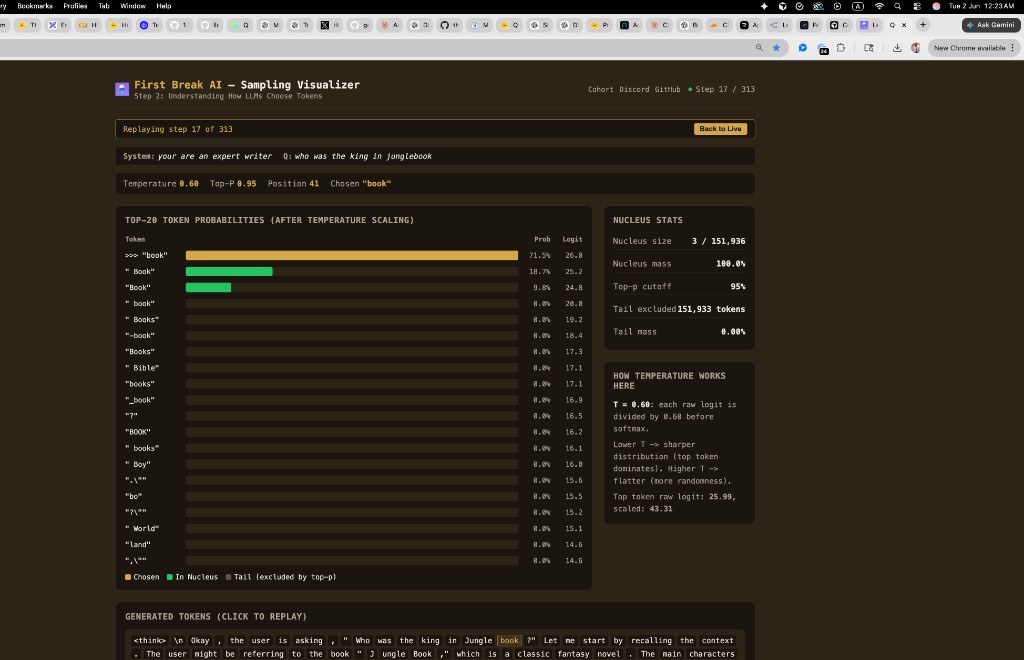
Quick read of the dashboard:
- Green bars = in the nucleus (eligible to be chosen)
- Grey bars = tail (excluded by top-p)
- Gold bar = the token that was actually sampled
- Nucleus mass shows the cumulative probability of all nucleus tokens
- Tail excluded shows how many of the 151,936 vocabulary tokens were cut
When an Unlikely Token Wins — Probability Is Chance, Not Destiny
Here is a real step from the sampling visualizer. The model was asked “who was the king in the jungle book” and at this decode step, with T=0.60 and top-p=0.95, the nucleus had 9 tokens:
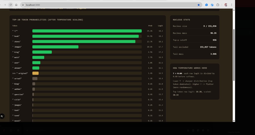
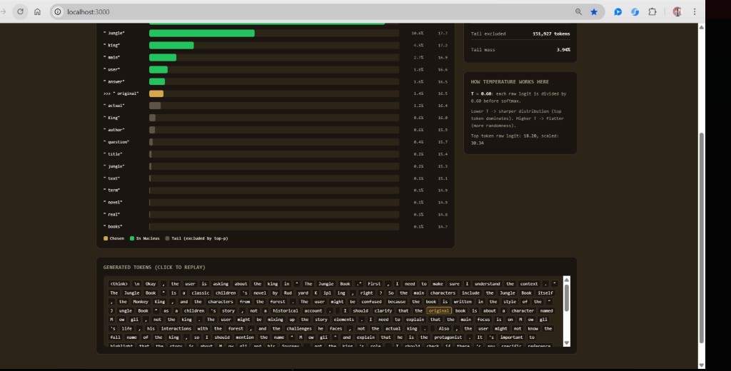
The natural question: why did ” original” win when ” book” was ~17x more likely?
The model does not always pick the highest-probability token. With default settings, it randomly samples from the nucleus. A 1.4% outcome is unlikely but valid — like drawing a rare ticket from a weighted lottery.
The Weighted Lottery
Imagine 100 tickets in a bag:
- ~25 tickets say
" \"" - ~25 say
" book" - ~24 say
" story" - ~1–2 say
" original"
You pull one ticket. Usually you get " book" or " story". Sometimes you get " original". That is stochastic sampling, not a bug.
The relevant code in sample_topp():
float r = coin * cumulative_prob;
float cdf = 0;
for (int i = 0; i <= last_idx; i++) {
    cdf += probindex[i].prob;
    if (r < cdf)
        return probindex[i].index;
}
The coin is a uniform random number in [0, 1). If it lands in the 1.4% slice belonging to " original", that token wins. Run the same prompt again with a different random seed and the model will likely pick " book" or " story" instead.
Why Not Always Pick the Top Token?
| Mode | Flag | Behavior |
|---|---|---|
| Greedy | -t 0 |
Always argmax — highest probability every time |
| Sampling | -t 0.6 (default) |
Weighted random — more natural, varied text |
| Top-p | -p 0.95 (default) |
Ignore the long tail so output stays coherent |
Greedy text can be repetitive and mechanical. Sampling trades a bit of unpredictability for variety — the same reason human writers don’t always pick the most obvious word. Top-p prevents sampling from the bottom 99.99% of unlikely tokens, so the output stays coherent even with randomness.
Experiments to Try
Run the bridge with different flags and watch how the dashboard changes:
# Sharper — top tokens win more often, fewer surprises
node ../../tools/sampling-bridge.mjs ./run_viz Qwen3-0.6B-FP32.gguf -v 1 -t 0.2 -p 0.95

# More surprises — flatter distribution, wider nucleus
node ../../tools/sampling-bridge.mjs ./run_viz Qwen3-0.6B-FP32.gguf -v 1 -t 1.2 -p 0.95

# Smaller nucleus — fewer candidates eligible
node ../../tools/sampling-bridge.mjs ./run_viz Qwen3-0.6B-FP32.gguf -v 1 -t 0.6 -p 0.5

# Always pick #1 (no lottery) — compare on the same prompt
./run Qwen3-0.6B-FP32.gguf -t 0
Seeing It Live — The Sampling Visualizer
The cohort has built a live dashboard that visualizes exactly what happens at every decode step. When you run the model with -v 1, each generated token emits a JSONL event containing the top-20 token probabilities, nucleus membership, and which token was chosen. You can replay any step and see the nucleus build up token by token.
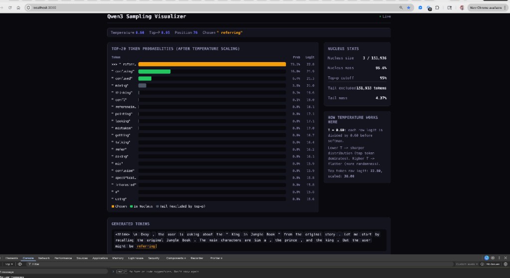
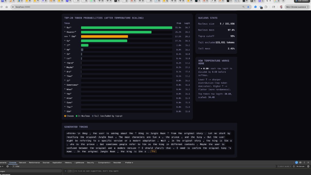
To run the visualizer yourself:
# Build the viz-enabled binary
make runviz

# Terminal 1: Start the dashboard
cd ../../apps/sampling-viz && npm install && npm run dev

# Terminal 2: Run inference with viz hook
node ../../tools/sampling-bridge.mjs ./run_viz Qwen3-0.6B-FP32.gguf -v 1 -t 0.6 -p 0.95
Then open http://localhost:3000 and chat in Terminal 2. Every generated token streams to the dashboard in real time.
What Top Labs Actually Use — Nucleus Sampling in Production
You’ve just learned nucleus sampling on a 0.6B model running on your laptop. Here’s the thing: this is the same sampling strategy that every major lab uses in production. Temperature + top-p (nucleus) is the universal default across the industry.
The Industry Landscape
| Lab / Model | Temperature | Top-p | Notes |
|---|---|---|---|
| OpenAI (GPT-4, etc.) | user-configurable | user-configurable | “Set one, not both” — they interact in hard-to-predict ways |
| OpenAI reasoning (o1, o3, o4-mini) | fixed at 1.0 | fixed at 1.0 | API rejects any attempt to change them |
| Anthropic (Claude) | user-configurable | user-configurable | Extended-thinking mode only allows top_p in 0.95–1.0 |
| Qwen3 (thinking mode) | 0.6 | 0.95 | “Do not use greedy decoding” — endless repetitions |
| Qwen3 (non-thinking) | 0.7 | 0.8 | Also uses top_k=20 and presence penalty=1.5 |
| DeepSeek-R1 | 0.6 | 0.95 | Benchmarks use 64 samples per prompt for pass@1 |
| DeepSeek-V3 | 1.0 (API) | 0.95 | Hidden mapping: T_internal = T_API × 0.3, so “1.0” is actually 0.3 |
| Kimi K2 (Moonshot AI) | 0.6 | — | API maps temperature: real_T = request_T × 0.6 |
Top-k has largely fallen out of favor at the API level because nucleus is adaptive — the cutoff expands when the model is uncertain, shrinks when it’s confident — while top-k is a static count regardless of the distribution shape.
A newer technique worth knowing: min-p sampling (ICLR 2025). It uses a relative threshold — keep any token whose probability is at least p × p_max — which behaves better than top-p at high temperatures, where flat distributions let top-p admit garbage tokens. Qwen3 has started reporting min-p in its recommended configs.
Why Reasoning Models Need Stochastic Sampling
This is the most important insight from the table above: reasoning models actively forbid greedy decoding.
OpenAI’s o1/o3 models fix temperature at 1.0 and reject API calls that try to change it. Qwen3’s docs warn explicitly: “Do not use greedy decoding, as it can lead to performance degradation and endless repetitions.”
The reason is the same for both: these models were trained with reinforcement learning to produce long self-correcting reasoning chains. The RL rollouts during training were generated with stochastic sampling, so the model learned to explore — “let me try X… wait, that doesn’t work because… let me reconsider…” — and that exploration depends on occasionally picking a non-top token.
Collapsing to greedy (-t 0) kills this. The model always takes the most probable next token, which means it can never deviate from its first idea, never self-correct, never explore alternative reasoning paths. The chain degenerates into repetition loops.
You can observe this directly with your visualizer:
-t 0.0(greedy): Watch the model get stuck repeating phrases. The gold bar is always on the top token — no exploration, no recovery from bad paths.-t 0.6(recommended): The top token still wins most of the time, but occasionally a second or third token wins. These are the moments where the model “changes its mind” mid-reasoning.-t 1.2(too hot): The distribution gets so flat that the model picks near-random tokens. Reasoning becomes incoherent.
The sweet spot at 0.6 means: mostly confident, but with enough noise to self-correct.
Why OpenAI Fixes at 1.0 but Qwen3 Recommends 0.6
This seems contradictory — both say “reasoning needs stochasticity,” but OpenAI locks temperature to 1.0 while Qwen3 recommends 0.6. Three possible reasons:
- Hidden rescaling. DeepSeek-V3 maps
T_API × 0.3internally; Kimi K2 mapsT_API × 0.6. OpenAI’s “1.0” might actually be ~0.3–0.6 inside the model. We don’t know because it’s closed-source. - Different RL training. Qwen3’s RL rollouts may have been generated at lower temperature, so the model learned to explore at 0.6 rather than 1.0.
- Quality tradeoff. At T=1.0 the reasoning chain explores more but also gets noisier. Qwen3 found 0.6 to be the sweet spot between “enough exploration for self-correction” and “not so much noise that chains go off the rails.”
The design philosophy also differs: OpenAI is paternalistic (prevents the footgun at the API level), while Qwen3 is open-source and trusts you to read the docs.
The Pattern Across the Industry
Once you line up all the labs, a consistent picture emerges:
- Production APIs: temperature + top-p (nucleus). Often “tune one, not both.”
- Reasoning/thinking modes: temperature pushed up (0.6–1.0), top_p kept high (0.95–1.0), greedy actively discouraged.
- Non-thinking instruct modes: temperature lower (0.6–0.7), top_p tighter (0.8), often a presence penalty added to suppress repetition.
- Benchmark reporting: many samples per prompt (DeepSeek-R1 uses 64 completions per query), averaged for pass@k.
- Pretraining ablations: greedy for reproducibility — deterministic results across runs.
The DeepSeek-R1 model card (arXiv 2501.12948) is the shortest, most explicit recipe — it shows the connection between nucleus sampling and pass@k evaluation in two paragraphs. The Qwen3 technical report (arXiv 2505.09388) publishes separate sampling configs for thinking vs non-thinking modes, directly relevant to what you’re running locally.
Why the Prefill/Decode Split Matters for the Viz
In the code, when viz is enabled, we copy the raw logits on every step (both prefill and decode) because sample() mutates the logits array in-place. But we only emit the visualization event during decode steps — prefill logits are discarded since we’re not choosing a token from them:
// copy raw logits before sample() mutates them (for viz)
float* raw_logits_copy = NULL;
if (viz) {
    raw_logits_copy = malloc(sampler->vocab_size * sizeof(float));
    memcpy(raw_logits_copy, logits, sampler->vocab_size * sizeof(float));
}

next = sample(sampler, logits);  // this mutates logits!
During decode, the copy is emitted and freed. During prefill, the copy is never emitted — so it must be freed separately to avoid a memory leak:
// free logits copy if not emitted (prefill steps)
if (raw_logits_copy) { free(raw_logits_copy); }
Without that line, every prefill step would leak ~600 KB (151,936 floats × 4 bytes). For a 100-token prompt, that’s 60 MB leaked before the first word appears.
This chapter introduced prefill, decode, sampling, and the viz as they relate to the model’s weight and memory pipeline. For the complete treatment — how to build and run run.c, what tokens are, how BPE tokenization works, chat templates, the transformer forward pass layer by layer, and the full chat loop — see the Step 2 guide: Run a Model Locally.
Chapter 17: The KV Cache — Why the Model Remembers
The Problem
When the model generates token 50, it needs to attend to all 49 previous tokens. That means computing the attention score between the current query and every past key, then weighting every past value. Without caching, you’d have to recompute K and V for all 49 tokens through all 28 layers — from scratch — just to generate one new token. Then for token 51, you’d recompute all 50. Then all 51 for token 52. The cost would be quadratic in the number of tokens generated.
The KV cache eliminates this waste. Every time the model processes a token, it stores that token’s key and value vectors in a persistent buffer. On the next step, it only computes K and V for the new token and reads all previous ones from the cache. One compute, then reuse forever.
Allocation — Two Giant Flat Arrays
The KV cache is allocated once at startup, sized for the maximum context length the model supports:
int kv_dim = p->n_kv_heads * p->head_dim;  // 8 * 128 = 1024

s->key_cache   = calloc(p->n_layers * p->seq_len * kv_dim, sizeof(float));
s->value_cache = calloc(p->n_layers * p->seq_len * kv_dim, sizeof(float));
For Qwen3-0.6B, the numbers are:
n_layers= 28seq_len= 40,960 (maximum context length)kv_dim= 1,024 (8 KV heads × 128 per head)
Each cache is 28 × 40,960 × 1,024 × 4 bytes = 4.7 GB. Both caches together = 9.4 GB. This is larger than the model weights themselves (2.4 GB). The KV cache is the reason GPU memory is the bottleneck in inference, not model size.
In practice, the cache only fills up to the actual sequence length used, but the memory is allocated for the maximum up front.
The Memory Layout
The cache is a 3D array flattened into a 1D buffer. Here’s how it’s organized:
key_cache (one contiguous block):

Layer 0:  [pos 0: 1024 floats][pos 1: 1024 floats]...[pos 40959: 1024 floats]
Layer 1:  [pos 0: 1024 floats][pos 1: 1024 floats]...[pos 40959: 1024 floats]
...
Layer 27: [pos 0: 1024 floats][pos 1: 1024 floats]...[pos 40959: 1024 floats]
To find the slot for layer l at position pos:
int loff = l * p->seq_len * kv_dim;   // jump to this layer's section
// then: loff + pos * kv_dim           // jump to this position's slot
The Write Step — Filling the Cache
At the start of each layer in the forward pass, the code sets the K and V pointers to point directly into the cache at the current position:
for (int l = 0; l < p->n_layers; l++) {
    int loff = l * p->seq_len * kv_dim;
    s->k = s->key_cache + loff + pos * kv_dim;
    s->v = s->value_cache + loff + pos * kv_dim;
Then the K and V matmuls write their results straight into the cache:
    matmul(s->k, s->xb, w->wk + l * layer_offset, p->dim, kv_dim);
    matmul(s->v, s->xb, w->wv + l * layer_offset, p->dim, kv_dim);
There is no separate “store to cache” step. The pointer s->k already is the cache slot. The matmul output goes directly into the right place. This is the same pointer-trick philosophy as memory_map_weights() from Chapter 6 — no copying, just pointing.
Here’s a visual of what happens as the model processes three tokens:
After pos=0 ("What"):
  key_cache layer 0:  [K₀ filled][empty][empty]...
  value_cache layer 0: [V₀ filled][empty][empty]...

After pos=1 ("is"):
  key_cache layer 0:  [K₀][K₁ filled][empty]...
  value_cache layer 0: [V₀][V₁ filled][empty]...

After pos=2 ("attention"):
  key_cache layer 0:  [K₀][K₁][K₂ filled]...
  value_cache layer 0: [V₀][V₁][V₂ filled]...
Each forward() call fills one column in the cache. During prefill, this happens for every prompt token. During decode, one column per generated token.
The Read Step — Attention Looks Back
After storing the current K and V, the attention mechanism reads back all previous positions. For each query head, the code loops over every position from 0 to pos:
for (int h = 0; h < p->n_heads; h++) {
    float* q = s->q + h * p->head_dim;
    float* att = s->att + h * p->seq_len;

    // Score: dot product of current Q with every past K
    for (int t = 0; t <= pos; t++) {
        float* k = s->key_cache + loff + t * kv_dim + (h / kv_mul) * p->head_dim;
        float score = 0;
        for (int i = 0; i < p->head_dim; i++)
            score += q[i] * k[i];
        att[t] = score / sqrtf(p->head_dim);
    }

    softmax(att, pos + 1);

    // Weighted sum: blend every past V using the attention weights
    float* xb3 = s->xb3 + h * p->head_dim;
    memset(xb3, 0, p->head_dim * sizeof(float));
    for (int t = 0; t <= pos; t++) {
        float* v = s->value_cache + loff + t * kv_dim + (h / kv_mul) * p->head_dim;
        float a = att[t];
        for (int i = 0; i < p->head_dim; i++)
            xb3[i] += a * v[i];
    }
}
Two loops, both 0..pos:
- Score loop — Compute the dot product of the current query with every past key. Divide by
√head_dimfor numerical stability. Then softmax to get attention weights. - Value loop — Weighted sum of all past values using those weights. The result is the “contextualised” representation of the current token.
Without the cache, both of these loops would require recomputing K and V for every past token through the full layer stack. With the cache, they just read from memory.
GQA in the Cache — Why h / kv_mul
Notice the expression (h / kv_mul) * p->head_dim in the cache read. This is Grouped Query Attention at work.
Qwen3-0.6B has 16 query heads but only 8 KV heads. The ratio kv_mul = n_heads / n_kv_heads = 2 means each KV head serves 2 query heads. Integer division groups them:
Query head h |
h / kv_mul |
KV head used |
|---|---|---|
| 0 | 0 | KV head 0 |
| 1 | 0 | KV head 0 |
| 2 | 1 | KV head 1 |
| 3 | 1 | KV head 1 |
| … | … | … |
| 14 | 7 | KV head 7 |
| 15 | 7 | KV head 7 |
This halves the KV cache size. Instead of storing 16 heads × 128 dims = 2,048 floats per position, we store 8 heads × 128 dims = 1,024 floats. For long contexts, this saves gigabytes.
Why Context Length Is Expensive
The attention loop for (int t = 0; t <= pos; t++) is the cost centre. At position 100, each head does 100 dot products. At position 10,000, it does 10,000. Across 16 heads and 28 layers, generating one token at position 10,000 requires:
16 heads × 28 layers × 10,000 dot products × 128 multiplies = ~573 million operationsThis is why:
- Long contexts are slow. Each new token gets more expensive as the conversation grows.
- KV cache memory grows linearly with context length. At position 10,000:
28 layers × 10,000 × 1,024 × 4 bytes × 2 caches = 2.2 GBof cache in use. - Production engines (vLLM, TensorRT-LLM) use techniques like paged attention (allocating cache in chunks rather than one giant block), KV cache compression, and multi-query attention (even fewer KV heads) to manage this cost.
The Cache Connects Prefill and Decode
Now the connection from Chapter 16 is complete:
- Prefill exists to build the KV cache. Each
forward()call during prefill fills one position’s K and V across all 28 layers. After a 200-token prompt, the cache has 200 rows filled — the model “remembers” the entire prompt. - Decode reads the cache on every step. Each generated token attends to everything in the cache — the entire prompt plus all previously generated tokens.
- Multi-turn with prefix caching reuses the cache from prior turns. If the first turn filled positions 0–199, the second turn starts at position 200 instead of reprocessing from scratch. This is what the
[Sep-01-25] Prefix cachingupdate in the codebase implements.
The KV cache is the single data structure that makes autoregressive generation practical. Without it, LLM inference would be orders of magnitude slower.
Exercises
Exercise 1: Calculate the Header Size Yourself
Using header.txt, verify the magic number 5,951,648. You’ll need the total file size and the last tensor’s offset + size.
Hint: TENSOR_310’s offset is 2,993,946,624. Its shape is [1024, 3072] with TYPE=0 (F32 = 4 bytes per element).
Exercise 2: Count the Parameters
Using the tensor shapes in header.txt, calculate the total number of parameters in the model. Group them by category:
- Embedding parameters (token_embd + output)
- Per-layer attention parameters (Q, K, V, O projections + norms) × 28
- Per-layer FFN parameters (up, gate, down + norm) × 28
- Global norms
Does your total match approximately 600 million?
Exercise 3: Predict the Layer Offset
The code uses layer_offset = 62923776/4. Verify this by calculating the total size (in bytes) of all 11 tensors in one block using the dimensions from header.txt.
Exercise 4: What Would Break?
Describe what would happen in each scenario:
- The GGUF file was regenerated with a different tokenizer (more vocabulary entries)
- Someone reordered the tensors in the GGUF to put FFN weights before attention weights
- The model was quantized to Q4_0 instead of F32
Exercise 5: Read the Forward Pass
Trace through the forward() function with a single token at position 0, layer 0 only. Write down the shape of every matrix multiplication (input dimensions × output dimensions).
Exercise 6: SafeTensors Header Size
A SafeTensors JSON header entry for one tensor looks roughly like this (about 120 characters):
"model.layers.0.self_attn.q_proj.weight":{"dtype":"BF16","shape":[2048,1024],"data_offsets":[0,4194304]},Estimate the JSON header size for a model with 311 tensors. Then compare that with the GGUF header size of 5,951,648 bytes. Why is the GGUF header so much larger, even though its binary format is more compact than JSON?
Exercise 7: Trace the Name Translation
Pick any three tensors from header.txt. For each one, trace backwards through all four naming levels:
- The
run.cstruct field name (e.g.,w->wq) - The
header.txtname (e.g.,BLK_0_ATTN_Q_WEIGHT) - The GGUF standard name (e.g.,
blk.0.attn_q.weight) - The original PyTorch/SafeTensors name (e.g.,
model.layers.0.self_attn.q_proj.weight)
Exercise 8: File Size Comparison
Calculate the file sizes for Qwen3-0.6B in each format:
- SafeTensors with BF16 (2 bytes per parameter)
- GGUF with F32 (4 bytes per parameter, what run.c uses)
- GGUF with Q4_K_M (approximately 0.56 bytes per parameter)
For each, estimate what percentage of the file is header/metadata vs actual weight data.
Exercise 9: Prefill Cost
A user types a 200-token prompt. How many forward() calls happen during prefill? How many during decode if the model generates 50 tokens? What is the total? Now imagine the user sends a follow-up message in multi-turn mode with 30 more tokens — with prefix caching, how many prefill calls does the second turn need?
Exercise 10: Nucleus Math
The model produces these top-5 probabilities after temperature scaling and softmax: [0.45, 0.25, 0.15, 0.08, 0.04]. With top_p = 0.95:
- Which tokens are in the nucleus?
- What is the nucleus mass?
- How many tokens from the 151,936-token vocabulary are excluded?
- If you lower
top_pto 0.7, which tokens remain in the nucleus?
Exercise 11: KV Cache Memory
Qwen3-0.6B has 28 layers, 8 KV heads, head_dim 128, and seq_len 40,960.
- Calculate the KV cache size per position (both keys and values, in bytes).
- After processing a 500-token prompt, how much cache memory is in use?
- At the full context length (40,960 tokens), how much total memory do the key and value caches consume?
- The model weights are 2.4 GB. At what context length does the KV cache exceed the model weights?
- If the model used full multi-head attention (16 KV heads instead of 8), what would the cache size be at full context? How much does GQA save?
Glossary
Activation: An intermediate result computed during the forward pass. Unlike weights, activations are different for every input and are computed (not stored in the file).
BF16 (bfloat16): A 16-bit floating-point format developed by Google Brain. It has the same exponent range as FP32 (8 bits) but fewer mantissa bits (7 vs 23). This makes it ideal for training — it can represent the same range of values as FP32, just with less precision. Most HuggingFace models are distributed in BF16.
BPE (Byte Pair Encoding): A tokenization algorithm that breaks text into subword units by iteratively merging the most frequent pair of adjacent tokens. Used by GPT-2, Qwen, and many other models.
FP32 (Float32): A 32-bit floating-point number format. Each weight takes 4 bytes. This is full precision — no information is lost.
GGUF (GGML Universal Format): The file format used by llama.cpp and related projects to store model weights, tokenizer data, and metadata in a single self-describing file. Succeeded older GGML and GGJT formats.
GQA (Grouped Query Attention): A variant of multi-head attention where multiple query heads share a single key/value head. Qwen3-0.6B has 16 query heads but only 8 KV heads (kv_mul = 2). In run.c, the expression (h / kv_mul) * head_dim routes query head pairs to the same KV cache slot, halving the cache size from 2,048 to 1,024 floats per position per layer.
Head Dimension: The dimensionality of each individual attention head. For Qwen3-0.6B, this is 128. Total attention dimension = n_heads × head_dim = 16 × 128 = 2048.
KV Cache: Two flat arrays (key_cache and value_cache), each sized n_layers × seq_len × kv_dim, that store previously computed key and value vectors during autoregressive generation. In run.c, the K/V pointers are set directly into the cache (s->k = s->key_cache + loff + pos * kv_dim), so matmul writes straight into the cache slot with no copy. The attention loop reads positions 0..pos from the cache to compute scores and weighted sums. Without the cache, each new token would require recomputing K and V for all previous positions from scratch.
Layer Offset: The distance (in floats or bytes) between the same tensor type in consecutive layers. Because all layers have identical structure, this is a constant.
Logits: The raw output scores of the model, one per vocabulary token. Before sampling, these are typically converted to probabilities via softmax.
Nucleus Sampling (Top-p): A sampling strategy that keeps only the smallest set of tokens whose cumulative probability exceeds a threshold p (typically 0.95). Prevents the model from ever choosing very low-probability tokens, even at high temperatures.
mmap (Memory Map): An operating system feature that maps a file into virtual memory, allowing the program to access file contents through pointer dereferencing without explicitly reading the file into a buffer.
Pickle: A Python serialization format that can store arbitrary Python objects, including executable code. Previously used for PyTorch model files (.bin, .pt). Replaced by SafeTensors due to security risks (arbitrary code execution during deserialization).
Prefill: The first phase of inference where the model processes every token of the user’s prompt sequentially, building up the KV cache. No text is generated during prefill. The duration of this phase determines TTFT.
Quantization: Reducing the precision of weights (e.g., from 32-bit float to 4-bit integer) to reduce file size and memory usage, at the cost of some accuracy.
Residual Connection: Adding the input of a layer directly to its output. This helps gradients flow during training and is a defining feature of the transformer architecture.
RMSNorm (Root Mean Square Normalization): A normalization technique that scales a vector by the inverse of its root mean square. Simpler and faster than LayerNorm. Used in Qwen3, LLaMA, and most modern LLMs.
RoPE (Rotary Position Embedding): A method for encoding position information by rotating the query and key vectors. The rotation angle depends on the token’s position and a frequency base (1,000,000 for Qwen3).
SafeTensors: A secure, minimal file format created by HuggingFace for storing tensor data. Uses a JSON header for metadata and a contiguous byte buffer for tensor data. Cannot execute code. Does not include model configuration or tokenizer data — only weights.
Sharding: Splitting a large model file across multiple smaller files. Both SafeTensors and GGUF support sharding. An index file maps tensor names to their respective shard files.
SwiGLU: An activation function used in the FFN layers. It combines the Swish (SiLU) activation with a gating mechanism: SwiGLU(x) = Swish(W_gate × x) × (W_up × x). Requires two separate projections (gate and up) instead of one.
Temperature: A scaling factor applied to logits before softmax. Lower temperature (e.g. 0.2) sharpens the distribution, making the top token dominate. Higher temperature (e.g. 1.5) flattens it, increasing randomness. Temperature 0 is greedy (always pick the highest).
Tensor: A multi-dimensional array of numbers. A 1D tensor is a vector, a 2D tensor is a matrix. Model weights are stored as tensors.
Tensor Name Mapping: The process of translating framework-specific tensor names (like PyTorch’s model.layers.0.self_attn.q_proj.weight) to standardized GGUF names (like blk.0.attn_q.weight). Handled by the conversion script’s mapping table.
TPS (Tokens Per Second): The decode-phase generation speed — how many tokens the model produces per second after the first token. Measured with -r 1 in run.c.
TTFT (Time to First Token): The time from submitting a prompt to receiving the first generated token. Measures prefill duration. Measured with -f 1 in run.c. In production engines, this is the primary latency metric.
Transformer: The neural network architecture underlying modern LLMs. Consists of repeated blocks of self-attention followed by feed-forward networks, with residual connections and normalization.
Companion reading
The Lesson 1: HuggingFace Beyond Upload is the prerequisite — it covers the three LLM intuitions, config.json, and running Qwen3 in pure C that this lesson builds on. The cohort blog post on Running Qwen3 0.6B in pure C is a deeper walk through what is inside the .gguf file. GGUF vs SafeTensors covers the weight-format comparison from a different angle. The QWEN3-RunLocally repo contains the run.c code referenced throughout this lesson.
Next steps
When you are ready, do four things. Read the run.c source code with this lesson open beside it — map every struct field back to its GGUF tensor name. Do the exercises above — especially Exercise 5, which will cement the forward-pass flow. Open modeling_qwen3.py and compare it to run.c side by side — they describe the same computation. And then continue to Step 2 on the Roadmap with a clear mental model of how bytes on disk become logits in memory.